生成数据集
import torch
import numpy as np
import math
from torch import nn
import matplotlib.pyplot as plt
from d2l import torch as d2l

max_degree = 20  # 我们最多用到 20 阶多项式
n_train, n_test = 100, 100  # 训练集和测试集各取 100 条样本
true_w = np.zeros(max_degree)  # 先把所有系数设为 0,后面再给前几项赋真实值
true_w[0:4] = np.array([5, 1.2, -3.4, 5.6])
print("[1/4] 初始化完成")
print(f"max_degree={max_degree}, n_train={n_train}, n_test={n_test}")
print(f"真实系数前6项: {true_w[:6]}")

features = np.random.normal(size=(n_train + n_test, 1))
np.random.shuffle(features)
print("[2/4] 原始特征生成完成")
print(f"features.shape={features.shape}")
print(f"features前2条: {features[:2].reshape(-1)}")

poly_features = np.power(features, np.arange(max_degree).reshape(1, -1))
for i in range(max_degree):
    poly_features[:, i] /= math.gamma(i + 1)  # 每一列除以 i!,避免高次项数值过大
print("[3/4] 多项式特征构造完成")
print(f"poly_features.shape={poly_features.shape}")
print(f"第1条样本前6维多项式特征: {poly_features[0, :6]}")

# labels 是一维向量,长度为 n_train + n_test
labels = np.dot(poly_features, true_w)
labels += np.random.normal(scale=0.1, size=labels.shape)
print("标签生成完成(含少量噪声)")
print(f"labels.shape={labels.shape}, mean={labels.mean():.4f}, std={labels.std():.4f}")
print(f"labels前3个值: {labels[:3]}")

# 把 NumPy 数组转成 PyTorch 张量,方便后续用深度学习框架训练
true_w, features, poly_features, labels = [torch.tensor(x, dtype=
    torch.float32) for x in [true_w, features, poly_features, labels]]
print("[4/4] 张量转换完成")
print(f"features.dtype={features.dtype}, poly_features.dtype={poly_features.dtype}, labels.dtype={labels.dtype}")
print(f"features前2条: {features[:2].reshape(-1)}")
print(f"poly_features前2条前6维: {poly_features[:2, :6]}")
print(f"labels前3个值: {labels[:2]}")
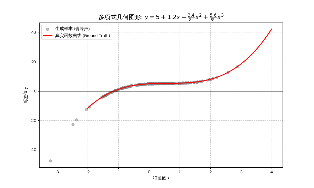
使用以下三阶多项式来生成训练和测试数据的标签:
\[y = 5 \cdot \frac{x^0}{0!} + 1.2 \cdot \frac{x^1}{1!} + (-3.4) \cdot \frac{x^2}{2!} + 5.6 \cdot \frac{x^3}{3!} + \epsilon\]阶乘定义 (Factorial)
\[n! = n \times (n-1) \times (n-2) \times \dots \times 1\]常见阶乘表
| n | n! | 计算方式 |
|---|---|---|
| 0 | 1 | 定义为 1 |
| 1 | 1 | 1 |
| 2 | 2 | 2 × 1 |
| 3 | 6 | 3 × 2 × 1 |
| 4 | 24 | 4 × 3 × 2 × 1 |
| 5 | 120 | 5 × 4 × 3 × 2 × 1 |
| 6 | 720 | 6 × 5 × 4 × 3 × 2 × 1 |
为什么要除阶乘
- 防止高次项数值爆炸
- 数值稳定
- 类似 泰勒展开
几何图形
当数据集只有10个数据时的运行结果,多项式是5阶的神经网络
# features(原始输入) :比如今天的温度
tensor([[-0.4639],  # 样本1的原始特征 x
        [-0.3173],  # 样本2的原始特征 x
        [ 0.4466],  # 样本3的原始特征 x
        [-0.0406],  # 样本4的原始特征 x
        [-0.1815],  # 样本5的原始特征 x
        [ 0.4002],  # 样本6的原始特征 x
        [-0.1662],  # 样本7的原始特征 x
        [ 1.0576],  # 样本8的原始特征 x
        [-0.7593],  # 样本9的原始特征 x
        [ 1.3801],  # 样本10的原始特征 x
        [-1.0304],  # 样本11的原始特征 x
        [-0.4161],  # 样本12的原始特征 x
        [ 0.2956],  # 样本13的原始特征 x
        [ 1.9887],  # 样本14的原始特征 x
        [-0.7561],  # 样本15的原始特征 x
        [ 1.3349],  # 样本16的原始特征 x
        [-0.3577],  # 样本17的原始特征 x
        [-1.3001],  # 样本18的原始特征 x
        [-1.7494],  # 样本19的原始特征 x
        [-0.0220]]) # 样本20的原始特征 x

# 多项式展开:     1       x          x²/2!     x³/3!      x⁴/4!
tensor([[ 1.000000, -0.463900,  0.107600, -0.016639,  0.001930],  # 样本1: [1, x, x²/2!, x³/3!, x⁴/4!]
        [ 1.000000, -0.317310,  0.050343, -0.005325,  0.000422],  # 样本2
        [ 1.000000,  0.446560,  0.099708,  0.014842,  0.001657],  # 样本3
        [ 1.000000, -0.040568,  0.000823, -0.000011,  0.000000],  # 样本4
        [ 1.000000, -0.181500,  0.016472, -0.000997,  0.000045],  # 样本5
        [ 1.000000,  0.400170,  0.080070,  0.010681,  0.001069],  # 样本6
        [ 1.000000, -0.166150,  0.013803, -0.000764,  0.000032],  # 样本7
        [ 1.000000,  1.057600,  0.559290,  0.197170,  0.052133],  # 样本8
        [ 1.000000, -0.759310,  0.288280, -0.072965,  0.013851],  # 样本9
        [ 1.000000,  1.380100,  0.952330,  0.438100,  0.151160],  # 样本10
        [ 1.000000, -1.030400,  0.530810, -0.182310,  0.046960],  # 样本11
        [ 1.000000, -0.416140,  0.086585, -0.012010,  0.001250],  # 样本12
        [ 1.000000,  0.295550,  0.043676,  0.004303,  0.000318],  # 样本13
        [ 1.000000,  1.988700,  1.977500,  1.310900,  0.651740],  # 样本14
        [ 1.000000, -0.756050,  0.285810, -0.072029,  0.013614],  # 样本15
        [ 1.000000,  1.334900,  0.890940,  0.396430,  0.132290],  # 样本16
        [ 1.000000, -0.357700,  0.063988, -0.007630,  0.000682],  # 样本17
        [ 1.000000, -1.300100,  0.845090, -0.366230,  0.119030],  # 样本18
        [ 1.000000, -1.749400,  1.530200, -0.892310,  0.390250],  # 样本19
        [ 1.000000, -0.022049,  0.000243, -0.000002,  0.000000]]) # 样本20

# 目标值 Y
tensor([ 3.9165,  # 样本1的 y = f(x) + noise
         4.5654,  # 样本2
         5.2743,  # 样本3
         4.9747,  # 样本4
         4.7755,  # 样本5
         5.1702,  # 样本6
         4.6201,  # 样本7
         5.3590,  # 样本8
         2.6294,  # 样本9
         5.7515,  # 样本10
         1.0478,  # 样本11
         4.2479,  # 样本12
         4.9853,  # 样本13
         8.0518,  # 样本14
         2.6496,  # 样本15
         5.8060,  # 样本16
         4.3129,  # 样本17
        -1.5026,  # 样本18
        -7.0915,  # 样本19
         4.8553]) # 样本20
| 数据 | 含义 | 形状 |
|---|---|---|
features |
原始输入 x | (20,1) |
poly_features |
多项式特征 | (20,5) |
labels |
真实输出 y | (20,) |
案例理解数据
| 步骤 | 生活类比 |
|---|---|
| features | 当天温度 |
| poly_features | 温度的各种组合:x, x², x³…(让模型学到非线性规律) |
| true_w | 冰淇淋销量规律(你脑子里想的经验公式) |
| labels | 真实销量(加上一点随机噪声) |
| 神经网络 | 根据温度预测销量的“智能员工” |
给神经网络的不是单纯的温度 x,而是温度的各种组合(poly_features),让它学到曲线规律,从而预测销量。
对模型进行训练和测试
def evaluate_loss(net, data_iter, loss):
"""评估给定数据集上模型的损失"""
# Accumulator(2):
# 第 0 位累计“总损失”;第 1 位累计“样本总数”。
metric = d2l.Accumulator(2) # 损失总和,样本数量
for X, y in data_iter:
# 前向计算预测值
out = net(X)
# 把标签形状调整成和输出一致,避免广播引发的形状问题
y = y.reshape(out.shape)
# 按样本计算损失(因为 reduction='none')
l = loss(out, y)
# 累计这一批的总损失和样本数
metric.add(l.sum(), l.numel())
# 返回“平均损失”
return metric[0] / metric[1]
def train_epoch_ch3(net, train_iter, loss, updater):
"""兼容版 train_epoch_ch3:训练模型一个 epoch 并返回平均损失。"""
if isinstance(net, nn.Module):
net.train()
metric = d2l.Accumulator(2) # 损失总和、样本数量
for X, y in train_iter:
y_hat = net(X)
l = loss(y_hat, y)
# 兼容两种更新器:PyTorch 优化器 / 自定义 updater 函数
if isinstance(updater, torch.optim.Optimizer):
updater.zero_grad()
l.mean().backward()
updater.step()
metric.add(float(l.sum()), y.numel())
else:
l.sum().backward()
updater(X.shape[0])
metric.add(float(l.sum()), y.numel())
return metric[0] / metric[1]
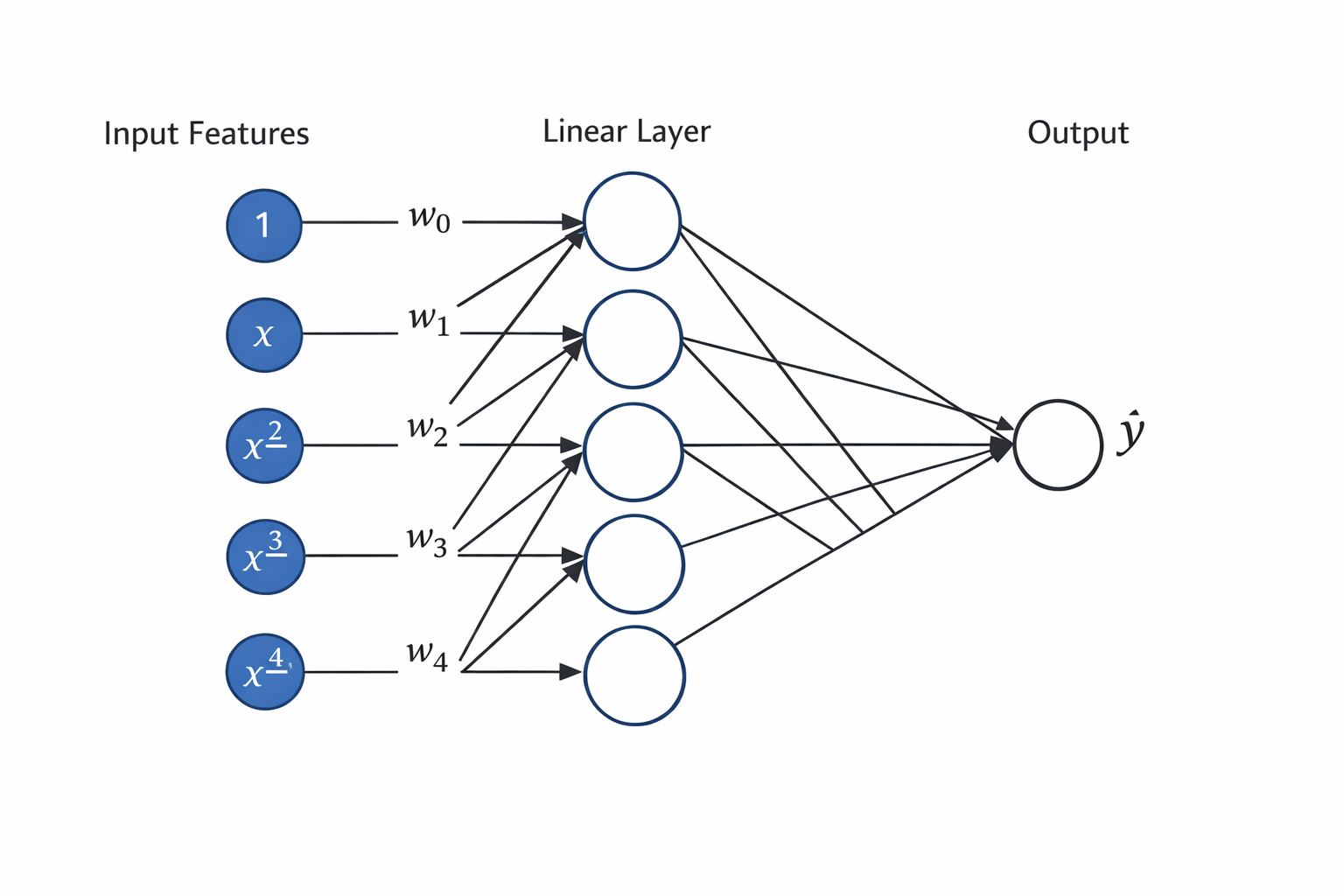
def train(train_features, test_features, train_labels, test_labels,
num_epochs=400):
# MSE 损失,先不做 batch 内平均,后面自己统计更直观
loss = nn.MSELoss(reduction='none')
# 输入维度等于每个样本的特征数(即多项式项数)
input_shape = train_features.shape[-1]
# 不设置偏置,因为我们已经在多项式中实现了它
# 这里的 x^0 特征恒为 1,等价于截距项(偏置)
net = nn.Sequential(nn.Linear(input_shape, 1, bias=False))
# 小批量大小不超过 10,也不超过训练样本总数
batch_size = min(10, train_labels.shape[0])
# 构建训练/测试迭代器
train_iter = d2l.load_array((train_features, train_labels.reshape(-1,1)),
batch_size)
test_iter = d2l.load_array((test_features, test_labels.reshape(-1,1)),
batch_size, is_train=False)
# 使用 SGD 优化器
trainer = torch.optim.SGD(net.parameters(), lr=0.01)
# 动态绘制训练集和测试集损失曲线(对数坐标)
animator = d2l.Animator(xlabel='epoch', ylabel='loss', yscale='log',
xlim=[1, num_epochs], ylim=[1e-3, 1e2],
legend=['train', 'test'])
# 训练主循环
for epoch in range(num_epochs):
# 训练一个 epoch(完成一遍训练集)
d2l.train_epoch_ch3(net, train_iter, loss, trainer)
# 第 1 轮和之后每 20 轮,记录一次训练/测试损失
if epoch == 0 or (epoch + 1) % 20 == 0:
animator.add(epoch + 1, (evaluate_loss(net, train_iter, loss),
evaluate_loss(net, test_iter, loss)))
# 打印学到的权重,观察是否接近真实系数
print('weight:', net[0].weight.data.numpy())
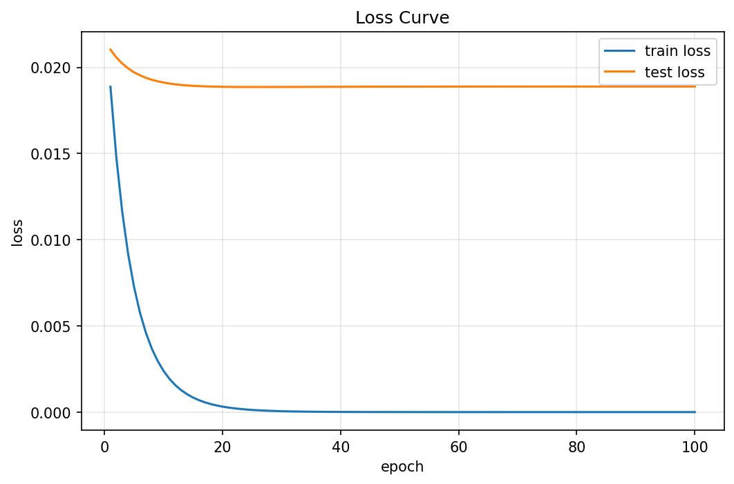
三阶多项式函数拟合(正常)
# 三阶多项式回归函数拟合(正常)
train(poly_features[:n_train, :4], poly_features[n_train:, :4],
      labels[:n_train], labels[n_train:])
运行结果
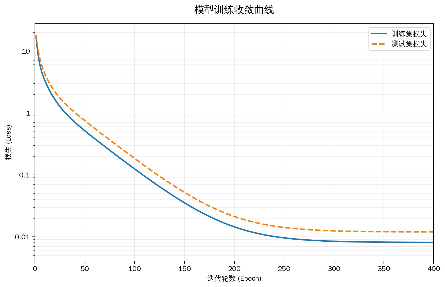
epoch   1: train_loss=17.460803, test_loss=18.468258
epoch  20: train_loss=1.656165, test_loss=2.210859
epoch  40: train_loss=0.710145, test_loss=1.023186
epoch  60: train_loss=0.384914, test_loss=0.563929
epoch  80: train_loss=0.217681, test_loss=0.321073
epoch 100: train_loss=0.125239, test_loss=0.185759
epoch 120: train_loss=0.073641, test_loss=0.108046
epoch 140: train_loss=0.044766, test_loss=0.066090
epoch 160: train_loss=0.028621, test_loss=0.042199
epoch 180: train_loss=0.019598, test_loss=0.028910
epoch 200: train_loss=0.014551, test_loss=0.021344
epoch 220: train_loss=0.011729, test_loss=0.017226
epoch 240: train_loss=0.010153, test_loss=0.014929
epoch 260: train_loss=0.009270, test_loss=0.013650
epoch 280: train_loss=0.008777, test_loss=0.012935
epoch 300: train_loss=0.008501, test_loss=0.012518
epoch 320: train_loss=0.008346, test_loss=0.012297
epoch 340: train_loss=0.008260, test_loss=0.012174
epoch 360: train_loss=0.008212, test_loss=0.012104
epoch 380: train_loss=0.008185, test_loss=0.012068
epoch 400: train_loss=0.008169, test_loss=0.012053

weight: [[ 4.9851832  1.1990807 -3.3752635  5.592799 ]]
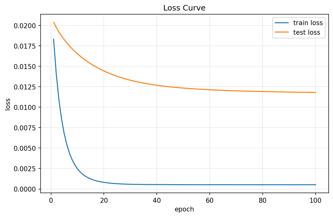
线性函数拟合(欠拟合)
train(poly_features[:n_train, :2], poly_features[n_train:, :2],
      labels[:n_train], labels[n_train:])
运行结果
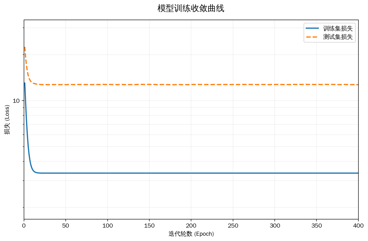
epoch   1: train_loss=13.030738, test_loss=22.471654
epoch  20: train_loss=3.360832, test_loss=12.744723
epoch  40: train_loss=3.358285, test_loss=12.737386
epoch  60: train_loss=3.358308, test_loss=12.731561
epoch  80: train_loss=3.358305, test_loss=12.731764
epoch 100: train_loss=3.358294, test_loss=12.757339
epoch 120: train_loss=3.358307, test_loss=12.731375
epoch 140: train_loss=3.358310, test_loss=12.766316
epoch 160: train_loss=3.358312, test_loss=12.731585
epoch 180: train_loss=3.358488, test_loss=12.707552
epoch 200: train_loss=3.358269, test_loss=12.748121
epoch 220: train_loss=3.358273, test_loss=12.747216
epoch 240: train_loss=3.358276, test_loss=12.754611
epoch 260: train_loss=3.358280, test_loss=12.757148
epoch 280: train_loss=3.358280, test_loss=12.739471
epoch 300: train_loss=3.358281, test_loss=12.747293
epoch 320: train_loss=3.358274, test_loss=12.743590
epoch 340: train_loss=3.358278, test_loss=12.756729
epoch 360: train_loss=3.358289, test_loss=12.757306
epoch 380: train_loss=3.358361, test_loss=12.722549
epoch 400: train_loss=3.358387, test_loss=12.718358

weight: [[3.8653178 2.6635108]]
高阶多项式函数拟合(过拟合)
# 从多项式特征中选取所有维度
train(poly_features[:n_train, :], poly_features[n_train:, :],
      labels[:n_train], labels[n_train:], num_epochs=1500)
运行结果
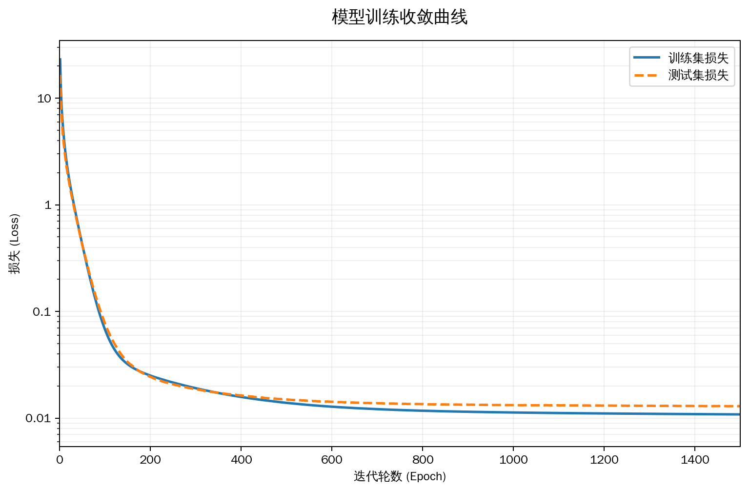
epoch   1: train_loss=23.100309, test_loss=16.543444
epoch  20: train_loss=1.835969, test_loss=1.689605
epoch  40: train_loss=0.663290, test_loss=0.644154
epoch  60: train_loss=0.271594, test_loss=0.284040
epoch  80: train_loss=0.124017, test_loss=0.136853
epoch 100: train_loss=0.067318, test_loss=0.076688
epoch 120: train_loss=0.044565, test_loss=0.050419
epoch 140: train_loss=0.034736, test_loss=0.037417
epoch 160: train_loss=0.029887, test_loss=0.030989
epoch 180: train_loss=0.027039, test_loss=0.026744
epoch 200: train_loss=0.025025, test_loss=0.024348
epoch 220: train_loss=0.023452, test_loss=0.022616
epoch 240: train_loss=0.022131, test_loss=0.021309
epoch 260: train_loss=0.020978, test_loss=0.020279
epoch 280: train_loss=0.019973, test_loss=0.019346
epoch 300: train_loss=0.019058, test_loss=0.018656
epoch 320: train_loss=0.018256, test_loss=0.017987
epoch 340: train_loss=0.017521, test_loss=0.017530
epoch 360: train_loss=0.016876, test_loss=0.017037
epoch 380: train_loss=0.016297, test_loss=0.016617
epoch 400: train_loss=0.015780, test_loss=0.016278
epoch 420: train_loss=0.015315, test_loss=0.015968
epoch 440: train_loss=0.014899, test_loss=0.015631
epoch 460: train_loss=0.014540, test_loss=0.015335
epoch 480: train_loss=0.014197, test_loss=0.015124
epoch 500: train_loss=0.013891, test_loss=0.014968
epoch 520: train_loss=0.013621, test_loss=0.014769
epoch 540: train_loss=0.013378, test_loss=0.014604
epoch 560: train_loss=0.013162, test_loss=0.014437
epoch 580: train_loss=0.012968, test_loss=0.014294
epoch 600: train_loss=0.012786, test_loss=0.014240
epoch 620: train_loss=0.012627, test_loss=0.014129
epoch 640: train_loss=0.012486, test_loss=0.013970
epoch 660: train_loss=0.012352, test_loss=0.013936
epoch 680: train_loss=0.012235, test_loss=0.013853
epoch 700: train_loss=0.012129, test_loss=0.013779
epoch 720: train_loss=0.012032, test_loss=0.013683
epoch 740: train_loss=0.011944, test_loss=0.013639
epoch 760: train_loss=0.011863, test_loss=0.013592
epoch 780: train_loss=0.011789, test_loss=0.013592
epoch 800: train_loss=0.011722, test_loss=0.013533
epoch 820: train_loss=0.011661, test_loss=0.013463
epoch 840: train_loss=0.011611, test_loss=0.013401
epoch 860: train_loss=0.011553, test_loss=0.013412
epoch 880: train_loss=0.011505, test_loss=0.013382
epoch 900: train_loss=0.011461, test_loss=0.013362
epoch 920: train_loss=0.011420, test_loss=0.013330
epoch 940: train_loss=0.011383, test_loss=0.013293
epoch 960: train_loss=0.011349, test_loss=0.013257
epoch 980: train_loss=0.011315, test_loss=0.013243
epoch 1000: train_loss=0.011285, test_loss=0.013227
epoch 1020: train_loss=0.011255, test_loss=0.013198
epoch 1040: train_loss=0.011229, test_loss=0.013179
epoch 1060: train_loss=0.011201, test_loss=0.013197
epoch 1080: train_loss=0.011177, test_loss=0.013193
epoch 1100: train_loss=0.011155, test_loss=0.013180
epoch 1120: train_loss=0.011132, test_loss=0.013180
epoch 1140: train_loss=0.011111, test_loss=0.013141
epoch 1160: train_loss=0.011091, test_loss=0.013132
epoch 1180: train_loss=0.011072, test_loss=0.013102
epoch 1200: train_loss=0.011053, test_loss=0.013091
epoch 1220: train_loss=0.011036, test_loss=0.013064
epoch 1240: train_loss=0.011018, test_loss=0.013058
epoch 1260: train_loss=0.011001, test_loss=0.013068
epoch 1280: train_loss=0.010985, test_loss=0.013039
epoch 1300: train_loss=0.010969, test_loss=0.013035
epoch 1320: train_loss=0.010954, test_loss=0.013012
epoch 1340: train_loss=0.010939, test_loss=0.013007
epoch 1360: train_loss=0.010924, test_loss=0.013004
epoch 1380: train_loss=0.010910, test_loss=0.013005
epoch 1400: train_loss=0.010896, test_loss=0.012987
epoch 1420: train_loss=0.010882, test_loss=0.012979
epoch 1440: train_loss=0.010869, test_loss=0.012943
epoch 1460: train_loss=0.010855, test_loss=0.012944
epoch 1480: train_loss=0.010842, test_loss=0.012941
epoch 1500: train_loss=0.010830, test_loss=0.012932
weight: [[ 4.9517536   1.2629199  -3.189622    5.3373904  -0.62576354  1.1583428
  -0.18633385  0.06696425  0.19166036  0.17446977 -0.036732    0.03489262
   0.10003854  0.17634493  0.01789237  0.07420919 -0.09644352  0.22096145
   0.07153416  0.12968667]]
什么是过拟合
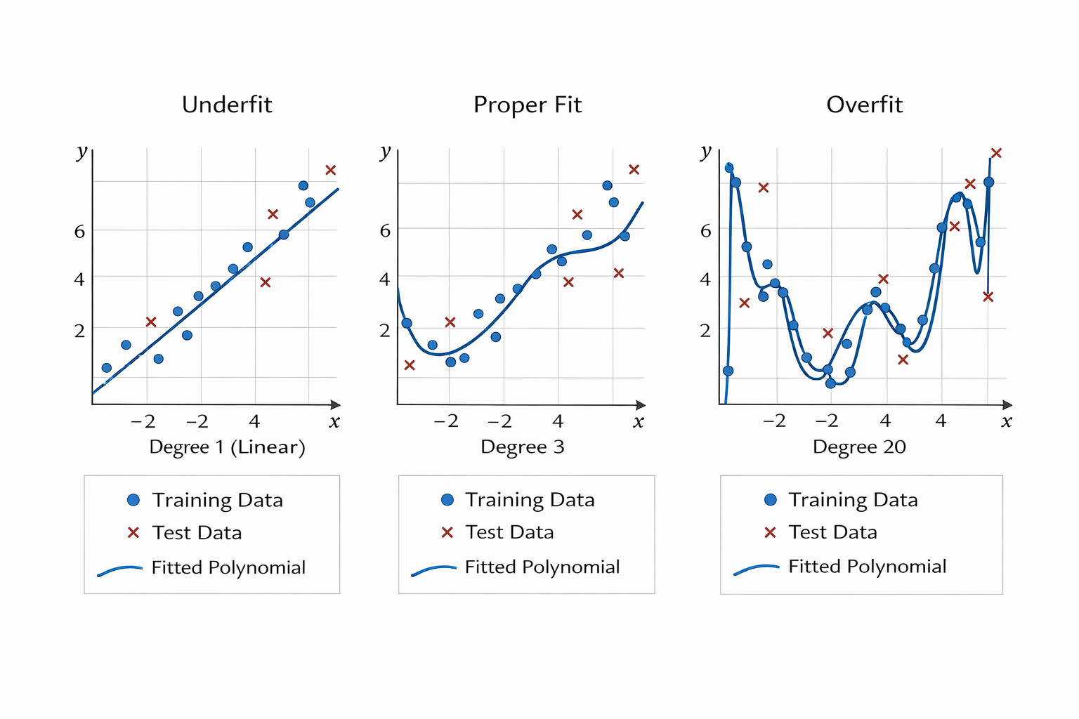
尝试使用一个阶数过高的多项式来训练模型。 在这种情况下,没有足够的数据用于学到高阶系数应该具有接近于零的值。因此,这个过于复杂的模型会轻易受到训练数据中噪声的影响。 虽然训练损失可以有效地降低,但测试损失仍然很高。
当阶数过高时,复杂模型对数据造成了过拟合:
训练数据有限:
- 你训练集只有 10 个样本
- 如果你用 20 阶多项式,你有 20 个权重要学
- 样本太少 → 权重学习不稳,会学到噪声
模型太灵活:
- 高阶多项式可以“弯曲”得非常复杂
- 它会尽量让预测 y 完全贴合训练数据,包括随机噪声
- 结果就是在训练集上误差很小,但在测试集上预测很差
噪声也被拟合:
- 你的 labels 含有随机噪声
- 高阶多项式可能把这些噪声也学进去
- 网络学到的 w_hat 不再接近真实 w,而是“曲线完全贴合训练点”
三种情况对比
权重衰减
权重衰减(Weight Decay)是机器学习中防止过拟合最常用的正则化技术之一。简单来说,它的核心思想是:在训练模型时,不仅要让预测更准,还要让模型的权重参数($w$)尽可能小。
为什么“权重小”能防止过拟合?
过拟合的模型:为了穿过每一个噪声点,权重往往会非常大。这导致函数在某些地方波动剧烈(斜率极大),对微小的输入变化产生巨大的输出波动。权重衰减后的模型:通过约束权重的大小,函数变得平滑。即使输入有一点点抖动,输出也不会剧烈跳变。
数学原理:给损失函数加个“紧箍咒”
在原始的损失函数 $L(\mathbf{w}, b)$ 后面,我们加上一个惩罚项(也叫正则项)。通常使用的是 L2 正则化:
\[L_{new} = L_{old} + \frac{\lambda}{2} \|\mathbf{w}\|^2\]- $|\mathbf{w}|^2$ 是所有权重平方的和。
- $\lambda$(超参数)控制惩罚的力度。$\lambda$ 越大,权重被压制得越厉害。
修改模型复杂度和权重衰减对比
为什么深度学习里“大模型 + 正则化”通常比“小模型”效果更好
| 特性 | 小模型(如 3 阶多项式) | 大模型(20 阶,无衰减) | 大模型 + 权重衰减(20 阶 + λ) | ||
|---|---|---|---|---|---|
| 核心逻辑 | 结构限制:直接砍掉不想要的特征。 | 完全自由:给所有特征完全的表达能力。 | 软性约束:保留结构,但增加权重的“使用成本”。 | ||
| 数学机制 | 减少参数数量。 | 允许所有参数自由增长。 | 在损失函数中加入 ( \lambda | w | ^2 )。 |
| 拟合能力 | 弱,容易欠拟合。 | 极强,甚至可以拟合噪声。 | 强,能抓主要趋势,同时不过度追踪噪声。 | ||
| 抗噪声能力 | 较好,因为模型看不见高阶细节。 | 很差,会把噪声当成真实规律。 | 最好,高阶权重会被自动压缩接近 0。 | ||
| 灵活性 | 低,阶数固定后难以适应更复杂数据。 | 很高,但容易“想太多”。 | 最高,可通过 λ 动态调整有效复杂度。 | ||
| 几何形态 | 曲线过于简单,可能漏掉真实转折。 | 曲线剧烈震荡,产生很多无意义波峰。 | 曲线平滑,更接近真实规律。 | ||
| 有效模型复杂度 | 固定复杂度。 | 极高复杂度。 | 自动复杂度控制。 | ||
| 工程实践 | 早期统计模型常见。 | 很少直接使用。 | 现代深度学习主流做法。 |
从零开始实现权重衰减案例
生成数据集
import torch
from torch import nn
from d2l import torch as d2l

# 样本规模与模型维度设置
# n_train: 训练样本数
# n_test: 测试样本数
# num_inputs: 特征维度(每条样本有 200 个特征)
# batch_size: 小批量训练时每批样本数
n_train, n_test, num_inputs, batch_size = 20, 100, 200, 5

# 构造“真实参数”,用于合成线性回归数据
# true_w: 权重向量,所有元素初始化为 0.01
# true_b: 偏置项
true_w, true_b = torch.ones((num_inputs, 1)) * 0.01, 0.05

# 生成训练集并打包为可迭代的小批量数据
train_data = d2l.synthetic_data(true_w, true_b, n_train)
train_iter = d2l.load_array(train_data, batch_size)

# 生成测试集;is_train=False 表示测试阶段不打乱数据
test_data = d2l.synthetic_data(true_w, true_b, n_test)
test_iter = d2l.load_array(test_data, batch_size, is_train=False)
初始化模型参数
def init_params():
    """初始化模型参数"""
    # 随机初始化权重,均值 0、标准差 0.01
    # requires_grad=True 表示后续训练时需要对其求梯度
    w = torch.normal(0, 0.01, size=(num_inputs, 1), requires_grad=True)
    # 偏置初始化为 0,同样需要参与梯度更新
    b = torch.zeros(1, requires_grad=True)
    return [w, b]
定义L2范数惩罚
def l2_penalty(w):
    """L2 正则化项"""
    # L2 正则常写作 ||w||^2 / 2,用于抑制权重过大,降低过拟合风险
    return torch.sum(w.pow(2)) / 2
定义训练代码实现
def train(lambd):
    """训练模型"""
    # 每次训练前重新初始化一组参数
    w, b = init_params()

    # 定义模型和损失函数:线性回归 + 平方损失
    net, loss = lambda X: d2l.linreg(X, w, b), d2l.squared_loss

    # 训练轮数和学习率
    num_epochs, lr = 100, 0.003

    # 训练主循环
    for epoch in range(num_epochs):
        # 遍历一个 epoch 内的所有小批量
        for X, y in train_iter:
            # 总损失 = 数据损失 + 正则项
            l = loss(net(X), y) + lambd * l2_penalty(w)

            # 反向传播计算梯度
            l.sum().backward()

            # 用小批量随机梯度下降更新参数
            d2l.sgd([w, b], lr, batch_size)

        # 评估阶段不需要记录梯度,节省内存并提升速度
        with torch.no_grad():
            # 在完整训练集/测试集上计算平均损失,观察拟合和泛化情况
            train_l = loss(net(train_data[0]), train_data[1])
            test_l = loss(net(test_data[0]), test_data[1])
            print(f'epoch {epoch + 1}, '
                  f'train loss {float(train_l.mean()):f}, '
                  f'test loss {float(test_l.mean()):f}')

    # 打印权重的 L2 范数,范数越大通常表示模型越复杂
    print('w的L2范数是:', torch.norm(w).item())
忽略正则化直接训练
train(lambd=0) # 不使用正则化
运行结果
训练后的偏置 b: 0.0039
真实偏置 true_b: 0.0500
训练后权重 w 的前10项:    [-0.0015  0.002  -0.0178 -0.001   0.0113 -0.0037 -0.0006  0.0127 -0.0172  -0.0033]
真实权重 true_w 的前10项: [0.01    0.01    0.01    0.01     0.01    0.01    0.01     0.01    0.01    0.01]
使用权重衰减
train(lambd=3) # 使用 L2 正则化
运行结果
w的L2范数是:0.0331
训练后的偏置 b: 0.0094
真实偏置 true_b: 0.0500
训练后权重 w 的前10项: [-0.00219  0.00137  0.00299 -0.00067 -0.00103  0.00113 -0.00105 -0.00053 -0.00226 -0.00218]
真实权重 true_w 的前10项: [0.01 0.01 0.01 0.01 0.01 0.01 0.01 0.01 0.01 0.01]
lambd参数调节
快速判断规则:
- 训练损失远小于测试损失:lambd 调大
- 训练和测试都高:lambd 调小
- 两者都低且接近:当前 lambd 比较合适
20训练样本
# 样本规模与模型维度设置
# n_train: 训练样本数
# n_test: 测试样本数
# num_inputs: 特征维度(每条样本有 200 个特征)
# batch_size: 小批量训练时每批样本数
n_train, n_test, num_inputs, batch_size = 20, 100, 200, 5
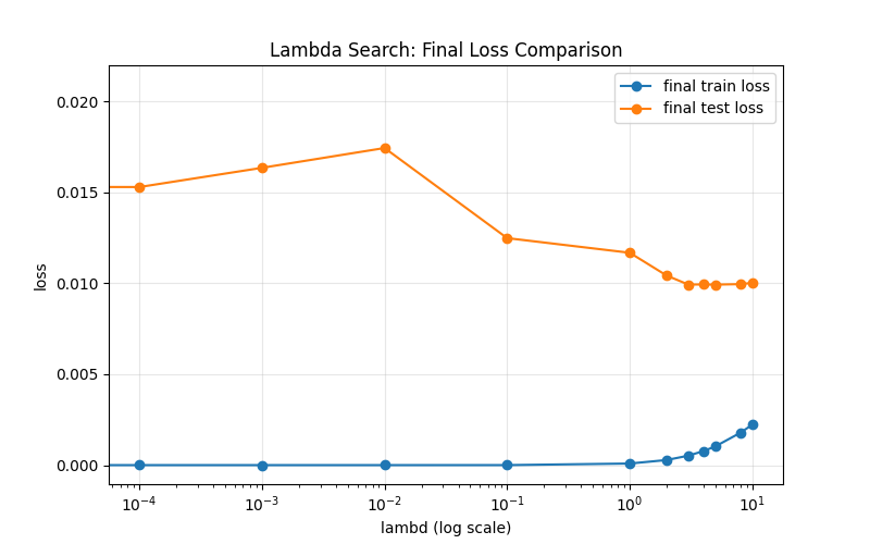
运行结果
===== 最佳 lambd =====
best lambd = 5
best final train loss = 0.001033
best final test loss = 0.009933
best w 的L2范数 = 0.0294
best 训练后的偏置 b: 0.0255
真实偏置 true_b: 0.0500
best 训练后权重 w 的前10项: [0.00149 0.00095 0.00256 0.00245 0.0018  0.00014 0.00439 0.0023  0.00214 0.00277]
真实权重 true_w 的前10项: [0.01 0.01 0.01 0.01 0.01 0.01 0.01 0.01 0.01 0.01]
100 训练样本
# 样本规模与模型维度设置
# n_train: 训练样本数
# n_test: 测试样本数
# num_inputs: 特征维度(每条样本有 200 个特征)
# batch_size: 小批量训练时每批样本数
n_train, n_test, num_inputs, batch_size = 100, 100, 200, 10
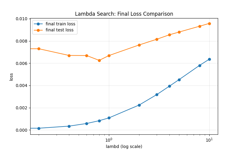
运行结果
===== 最佳 lambd =====
best lambd = 0.8
best final train loss = 0.000831
best final test loss = 0.006255
best w 的L2范数 = 0.0706
best 训练后的偏置 b: 0.0532
真实偏置 true_b: 0.0500
best 训练后权重 w 的前10项: [ 0.00114 -0.00618  0.00723  0.00372  0.00656 -0.00258  0.01001  0.00357 0.00406  0.00077]
真实权重 true_w 的前10项: [0.01 0.01 0.01 0.01 0.01 0.01 0.01 0.01 0.01 0.01]
0
次点赞