汇聚层
卷积神经网络(CNN)里的汇聚层(Pooling Layer),本质上可以理解为:对局部区域做“信息压缩 + 抗干扰”的操作
import torch
from torch import nn
from d2l import torch as d2l

# 手写二维池化函数,用于演示池化层的核心计算过程
# X: 输入的二维张量(可理解为单通道特征图)
# pool_size: 池化窗口大小,格式为(窗口高, 窗口宽)
# mode: 池化模式,'max'表示最大池化,'avg'表示平均池化
def pool2d(X, pool_size, mode='max'):
    # 从池化窗口尺寸中拆出高和宽
    p_h, p_w = pool_size

    # 计算输出特征图大小:
    # 不使用填充(padding)、步幅默认为1时,输出高 = 输入高 - 窗口高 + 1,宽同理
    Y = torch.zeros((X.shape[0] - p_h + 1, X.shape[1] - p_w + 1))

    # 遍历输出张量的每一个位置
    # 输出位置(i, j)对应输入中的一个局部窗口 X[i:i+p_h, j:j+p_w]
    for i in range(Y.shape[0]):
        for j in range(Y.shape[1]):
            # 最大池化:取该窗口中的最大值
            if mode == 'max':
                Y[i, j] = X[i:i + p_h, j:j + p_w].max()
            # 平均池化:取该窗口中的平均值
            elif mode == 'avg':
                Y[i, j] = X[i:i + p_h, j:j + p_w].mean()

    # 返回池化结果
    return Y

# 构造一个3x3输入张量,元素按行递增,便于直观看池化结果
X = torch.tensor([[0.0, 1.0, 2.0], [3.0, 4.0, 5.0], [6.0, 7.0, 8.0]])

print("输入张量 X:")
print(X)

# 使用2x2窗口做最大池化,并打印输出
# 该示例会得到2x2结果,每个元素是对应2x2局部区域的最大值
print("最大池化结果:")
print(pool2d(X, (2, 2)))

# 使用2x2窗口做平均池化,并打印输出
# 该示例会得到2x2结果,每个元素是对应2x2局部区域的平均值
print("平均池化结果:")
print(pool2d(X, (2, 2), mode='avg'))
运行结果
输入张量 X:
tensor([[0., 1., 2.],
        [3., 4., 5.],
        [6., 7., 8.]])
最大池化结果:
tensor([[4., 5.],
        [7., 8.]])
平均池化结果:
tensor([[2., 3.],
        [5., 6.]])
填充和步幅
# 下面演示 PyTorch 内置池化层 nn.MaxPool2d 的用法
# 构造 4x4 输入,并补齐 batch 与 channel 维度,形状为 (N, C, H, W) = (1, 1, 4, 4)
X = torch.arange(16, dtype=torch.float32).reshape(1, 1, 4, 4)
print("输入张量 X:")
print(X)

# 定义最大池化层:
# kernel_size=3:窗口大小 3x3
# padding=1:输入四周补 1 圈 0
# stride=2:窗口每次移动 2 个像素
pool2d = nn.MaxPool2d(3, padding=1, stride=2)

# 为了直观展示 padding=1 的效果,这里先手动打印补零后的输入张量
X_padded = nn.functional.pad(X, pad=(1, 1, 1, 1), mode='constant', value=0)
print("padding=1 后的张量 X_padded:")
print(X_padded)

# 执行池化,得到输出 Y
Y = pool2d(X)
print("使用 nn.MaxPool2d 进行池化后的结果 Y:")
print(Y)
运行结果
输入张量 X:
tensor([[[[ 0.,  1.,  2.,  3.],
          [ 4.,  5.,  6.,  7.],
          [ 8.,  9., 10., 11.],
          [12., 13., 14., 15.]]]])
padding=1 后的张量 X_padded:
tensor([[[[ 0.,  0.,  0.,  0.,  0.,  0.],
          [ 0.,  0.,  1.,  2.,  3.,  0.],
          [ 0.,  4.,  5.,  6.,  7.,  0.],
          [ 0.,  8.,  9., 10., 11.,  0.],
          [ 0., 12., 13., 14., 15.,  0.],
          [ 0.,  0.,  0.,  0.,  0.,  0.]]]])
使用 nn.MaxPool2d 进行池化后的结果 Y:
tensor([[[[ 5.,  7.],
          [13., 15.]]]])
多个通道
# 下面演示 PyTorch 内置池化层 nn.MaxPool2d 的用法
# 构造 4x4 输入,并补齐 batch 与 channel 维度,形状为 (N, C, H, W) = (1, 1, 4, 4)
X = torch.arange(16, dtype=torch.float32).reshape(1, 1, 4, 4)
print("输入张量 X:")
print(X)

X = torch.cat((X, X + 1), 1)  # 扩展到两个样本,形状变为 (2, 1, 4, 4)
print("扩展到两个样本后的输入张量 X:")
print(X)

pool2d = nn.MaxPool2d(3, padding=1, stride=2)
Y = pool2d(X)
print("使用 nn.MaxPool2d 进行池化后的结果 Y:")
print(Y)
运行结果
输入张量 X:
tensor([[[[ 0.,  1.,  2.,  3.],
          [ 4.,  5.,  6.,  7.],
          [ 8.,  9., 10., 11.],
          [12., 13., 14., 15.]]]])
扩展到两个样本后的输入张量 X:
tensor([[[[ 0.,  1.,  2.,  3.],
          [ 4.,  5.,  6.,  7.],
          [ 8.,  9., 10., 11.],
          [12., 13., 14., 15.]],

         [[ 1.,  2.,  3.,  4.],
          [ 5.,  6.,  7.,  8.],
          [ 9., 10., 11., 12.],
          [13., 14., 15., 16.]]]])
使用 nn.MaxPool2d 进行池化后的结果 Y:
tensor([[[[ 5.,  7.],
          [13., 15.]],

         [[ 6.,  8.],
          [14., 16.]]]])
卷积神经网络 LeNet
LeNet 是最早成功应用的卷积神经网络之一,由 Yann LeCun 在 1990 年代提出,主要用于手写数字识别(比如邮政编码)。
现代 CNN(如 YOLO、ResNet)的“祖师爷”
模型训练
# -*- coding: utf-8 -*-
import torch
from torch import nn
from d2l import torch as d2l
import matplotlib.pyplot as plt

# 使用 nn.Sequential 搭建经典 LeNet 风格网络:
# 输入是 Fashion-MNIST 的灰度图,形状为 (N, 1, 28, 28)
# 网络结构:卷积 -> 激活 -> 池化 -> 卷积 -> 激活 -> 池化 -> 展平 -> 全连接分类
net = nn.Sequential(
    # 第一层卷积:输入通道 1,输出通道 6,卷积核 5x5,padding=2 保持空间尺寸不变(28x28 -> 28x28)
    nn.Conv2d(1, 6, kernel_size=5, padding=2), nn.Sigmoid(),
    # 平均池化:窗口 2x2,步幅 2,尺寸减半(28x28 -> 14x14)
    nn.AvgPool2d(kernel_size=2, stride=2),
    # 第二层卷积:输入通道 6,输出通道 16,卷积核 5x5,不加 padding(14x14 -> 10x10)
    nn.Conv2d(6, 16, kernel_size=5), nn.Sigmoid(),
    # 第二次平均池化:尺寸再次减半(10x10 -> 5x5)
    nn.AvgPool2d(kernel_size=2, stride=2),
    # 展平为二维张量,供全连接层使用:(N, 16, 5, 5) -> (N, 16*5*5)
    nn.Flatten(),
    # 三层全连接:分类头,最终输出 10 类 logits
    nn.Linear(16 * 5 * 5, 120), nn.Sigmoid(),
    nn.Linear(120, 84), nn.Sigmoid(),
    nn.Linear(84, 10))

# 用随机输入做一次前向传播,仅打印每一层输入与输出的形状
X_demo = torch.rand(size=(1, 1, 28, 28), dtype=torch.float32)
for idx, layer in enumerate(net):
    X_in = X_demo
    X_out = layer(X_in)
    print(f'layer {idx + 1}: {layer.__class__.__name__}')
    print('input shape:\t', X_in.shape)
    print('output shape:\t', X_out.shape)
    print('-' * 80)
    X_demo = X_out

# 准备数据集迭代器
# batch_size 越大,吞吐通常越高,但会占用更多显存
batch_size = 256
train_iter, test_iter = d2l.load_data_fashion_mnist(batch_size = batch_size)

def evaluate_accuracy_gpu(net, data_iter, device=None): #@save
    """使用GPU计算模型在数据集上的精度"""
    if isinstance(net, nn.Module):
        net.eval()  # 设置为评估模式
        if not device:
            device = next(iter(net.parameters())).device
    # 正确预测的数量,总预测的数量
    metric = d2l.Accumulator(2)
    with torch.no_grad():
        for X, y in data_iter:
            if isinstance(X, list):
                # BERT微调所需的(之后将介绍)
                X = [x.to(device) for x in X]
            else:
                X = X.to(device)
            y = y.to(device)
            metric.add(d2l.accuracy(net(X), y), y.numel())
    return metric[0] / metric[1]

#@save
def train_ch6(net, train_iter, test_iter, num_epochs, lr, device):
    """用GPU训练模型(在第六章定义)"""
    # 参数初始化:对线性层与卷积层采用 Xavier 均匀分布初始化
    # 该初始化有助于在训练初期保持较稳定的信号方差,缓解梯度消失/爆炸
    def init_weights(m):
        if type(m) == nn.Linear or type(m) == nn.Conv2d:
            nn.init.xavier_uniform_(m.weight)
    net.apply(init_weights)

    # 将模型搬到指定设备(GPU 或 CPU)
    print('training on', device)
    net.to(device)

    # 优化器与损失函数:
    # - SGD:随机梯度下降
    # - CrossEntropyLoss:多分类交叉熵(输入应为未归一化 logits)
    optimizer = torch.optim.SGD(net.parameters(), lr=lr)
    loss = nn.CrossEntropyLoss()

    # timer 用于统计训练吞吐,num_batches 表示每个 epoch 的批次数
    timer, num_batches = d2l.Timer(), len(train_iter)
    train_loss_history, train_acc_history, test_acc_history = [], [], []
    for epoch in range(num_epochs):
        # 训练损失之和,训练准确率之和,样本数
        metric = d2l.Accumulator(3)
        net.train()
        for i, (X, y) in enumerate(train_iter):
            timer.start()
            # 梯度清零(PyTorch 默认梯度累加)
            optimizer.zero_grad()

            # 将当前批次数据放到同一设备上
            X, y = X.to(device), y.to(device)

            # 前向传播 -> 计算损失 -> 反向传播 -> 参数更新
            y_hat = net(X)
            l = loss(y_hat, y)
            l.backward()
            optimizer.step()

            # 在不记录梯度的模式下累积统计量,降低额外开销
            with torch.no_grad():
                # l * batch_size:把“平均损失”恢复成“总损失”,便于后续按样本数求平均
                metric.add(l * X.shape[0], d2l.accuracy(y_hat, y), X.shape[0])
            timer.stop()
            train_l = metric[0] / metric[2]
            train_acc = metric[1] / metric[2]

        # 每个 epoch 结束后在测试集上评估一次
        test_acc = evaluate_accuracy_gpu(net, test_iter)
        train_loss_history.append(float(train_l))
        train_acc_history.append(float(train_acc))
        test_acc_history.append(float(test_acc))

    # 训练结束后输出最终指标与吞吐信息
    print(f'loss {train_l:.3f}, train acc {train_acc:.3f}, '
          f'test acc {test_acc:.3f}')
    print(f'{metric[2] * num_epochs / timer.sum():.1f} examples/sec '
          f'on {str(device)}')
    epochs = list(range(1, num_epochs + 1))
    plt.figure(figsize=(8, 5))
    plt.plot(epochs, train_loss_history, label='train loss')
    plt.plot(epochs, train_acc_history, label='train acc')
    plt.plot(epochs, test_acc_history, label='test acc')
    plt.xlabel('epoch')
    plt.title('Training Curve')
    plt.legend()
    plt.grid(True, linestyle='--', alpha=0.4)
    plt.tight_layout()
    curve_path = '/home/lxg/code/AI/code/20260331/training_curve.png'
    plt.savefig(curve_path, dpi=150)
    plt.close()
    print('training curve saved to:', curve_path)
    for name, param in net.named_parameters():
        print(f'{name}: shape={tuple(param.shape)}')
        print(param.detach().cpu().flatten()[:10])

# 训练超参数:学习率与训练轮数
lr, num_epochs = 0.9, 10
# 启动训练,d2l.try_gpu() 会优先选择可用 GPU,否则退回 CPU
train_ch6(net, train_iter, test_iter, num_epochs, lr, d2l.try_gpu())
运行结果
layer 1: Conv2d
input shape: torch.Size([1, 1, 28, 28])
output shape: torch.Size([1, 6, 28, 28])
--------------------------------------------------------------------------------
layer 2: Sigmoid
input shape: torch.Size([1, 6, 28, 28])
output shape: torch.Size([1, 6, 28, 28])
--------------------------------------------------------------------------------
layer 3: AvgPool2d
input shape: torch.Size([1, 6, 28, 28])
output shape: torch.Size([1, 6, 14, 14])
--------------------------------------------------------------------------------
layer 4: Conv2d
input shape: torch.Size([1, 6, 14, 14])
output shape: torch.Size([1, 16, 10, 10])
--------------------------------------------------------------------------------
layer 5: Sigmoid
input shape: torch.Size([1, 16, 10, 10])
output shape: torch.Size([1, 16, 10, 10])
--------------------------------------------------------------------------------
layer 6: AvgPool2d
input shape: torch.Size([1, 16, 10, 10])
output shape: torch.Size([1, 16, 5, 5])
--------------------------------------------------------------------------------
layer 7: Flatten
input shape: torch.Size([1, 16, 5, 5])
output shape: torch.Size([1, 400])
--------------------------------------------------------------------------------
layer 8: Linear
input shape: torch.Size([1, 400])
output shape: torch.Size([1, 120])
--------------------------------------------------------------------------------
layer 9: Sigmoid
input shape: torch.Size([1, 120])
output shape: torch.Size([1, 120])
--------------------------------------------------------------------------------
layer 10: Linear
input shape: torch.Size([1, 120])
output shape: torch.Size([1, 84])
--------------------------------------------------------------------------------
layer 11: Sigmoid
input shape: torch.Size([1, 84])
output shape: torch.Size([1, 84])
--------------------------------------------------------------------------------
layer 12: Linear
input shape: torch.Size([1, 84])
output shape: torch.Size([1, 10])
--------------------------------------------------------------------------------
training on cuda:0
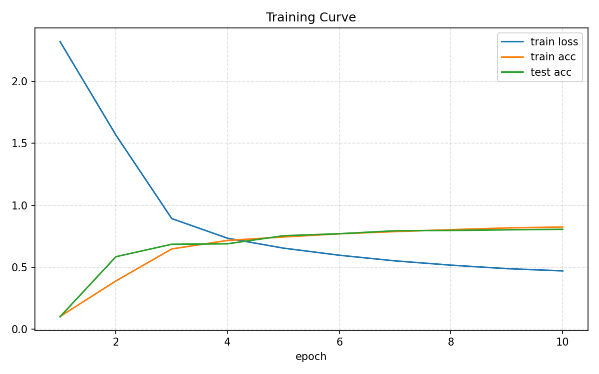
loss 0.470, train acc 0.824, test acc 0.805
148824.1 examples/sec on cuda:0
training curve saved to: /home/lxg/code/AI/code/20260331/training_curve.png
0.weight: shape=(6, 1, 5, 5)
tensor([-0.6876, 0.1083, 0.6188, 0.4408, -0.5378, -0.7944, 0.2383, 1.3344,
1.0854, -0.0504])
0.bias: shape=(6,)
tensor([-0.4167, 0.7430, 0.8318, -0.9601, -0.1775, 0.0031])
3.weight: shape=(16, 6, 5, 5)
tensor([0.1217, 0.4146, 0.5636, 0.4889, 0.1575, 0.1878, 0.3390, 0.3905, 0.3019,
0.1347])
3.bias: shape=(16,)
tensor([-0.0638, -0.0469, -0.1312, -0.0701, -0.2536, -0.0918, -0.1725, 0.1425,
-0.0381, 0.0242])
7.weight: shape=(120, 400)
tensor([ 0.1517, -0.0744, 0.0068, -0.0219, 0.1588, -0.0097, 0.0508, 0.1004,
0.0208, 0.0286])
7.bias: shape=(120,)
tensor([-0.0147, -0.0740, 0.0079, 0.0631, -0.0102, -0.0189, -0.0028, -0.0114,
-0.0170, -0.0336])
9.weight: shape=(84, 120)
tensor([-0.2921, 0.3081, -0.4017, -0.0009, 0.0037, 0.2289, -0.0957, -0.2042,
0.2774, 0.0443])
9.bias: shape=(84,)
tensor([ 0.0002, -0.0706, -0.0529, -0.0467, -0.1499, -0.1127, -0.0587, -0.0876,
-0.0610, -0.1212])
11.weight: shape=(10, 84)
tensor([-0.6706, 0.7223, 1.0911, -0.0302, -0.0456, 0.0688, -0.3650, 0.1078,
-0.3081, 0.0899])
11.bias: shape=(10,)
tensor([-0.0804, 0.2046, 0.3040, -0.1074, 0.0757, -0.0337, 0.1194, -0.2057,
-0.1287, -0.5384])
训练曲线
每层的解释
# 使用 nn.Sequential 搭建经典 LeNet 风格网络:
# 输入是 Fashion-MNIST 的灰度图,形状为 (N, 1, 28, 28)
# 网络结构:卷积 -> 激活 -> 池化 -> 卷积 -> 激活 -> 池化 -> 展平 -> 全连接分类
net = nn.Sequential(
    # 第一层卷积:输入通道 1,输出通道 6,卷积核 5x5,padding=2 保持空间尺寸不变(28x28 -> 28x28)
    nn.Conv2d(1, 6, kernel_size=5, padding=2), nn.Sigmoid(),
    # 平均池化:窗口 2x2,步幅 2,尺寸减半(28x28 -> 14x14)
    nn.AvgPool2d(kernel_size=2, stride=2),
    # 第二层卷积:输入通道 6,输出通道 16,卷积核 5x5,不加 padding(14x14 -> 10x10)
    nn.Conv2d(6, 16, kernel_size=5), nn.Sigmoid(),
    # 第二次平均池化:尺寸再次减半(10x10 -> 5x5)
    nn.AvgPool2d(kernel_size=2, stride=2),
    # 展平为二维张量,供全连接层使用:(N, 16, 5, 5) -> (N, 16*5*5)
    nn.Flatten(),
    # 三层全连接:分类头,最终输出 10 类 logits
    nn.Linear(16 * 5 * 5, 120), nn.Sigmoid(),
    nn.Linear(120, 84), nn.Sigmoid(),
    nn.Linear(84, 10))
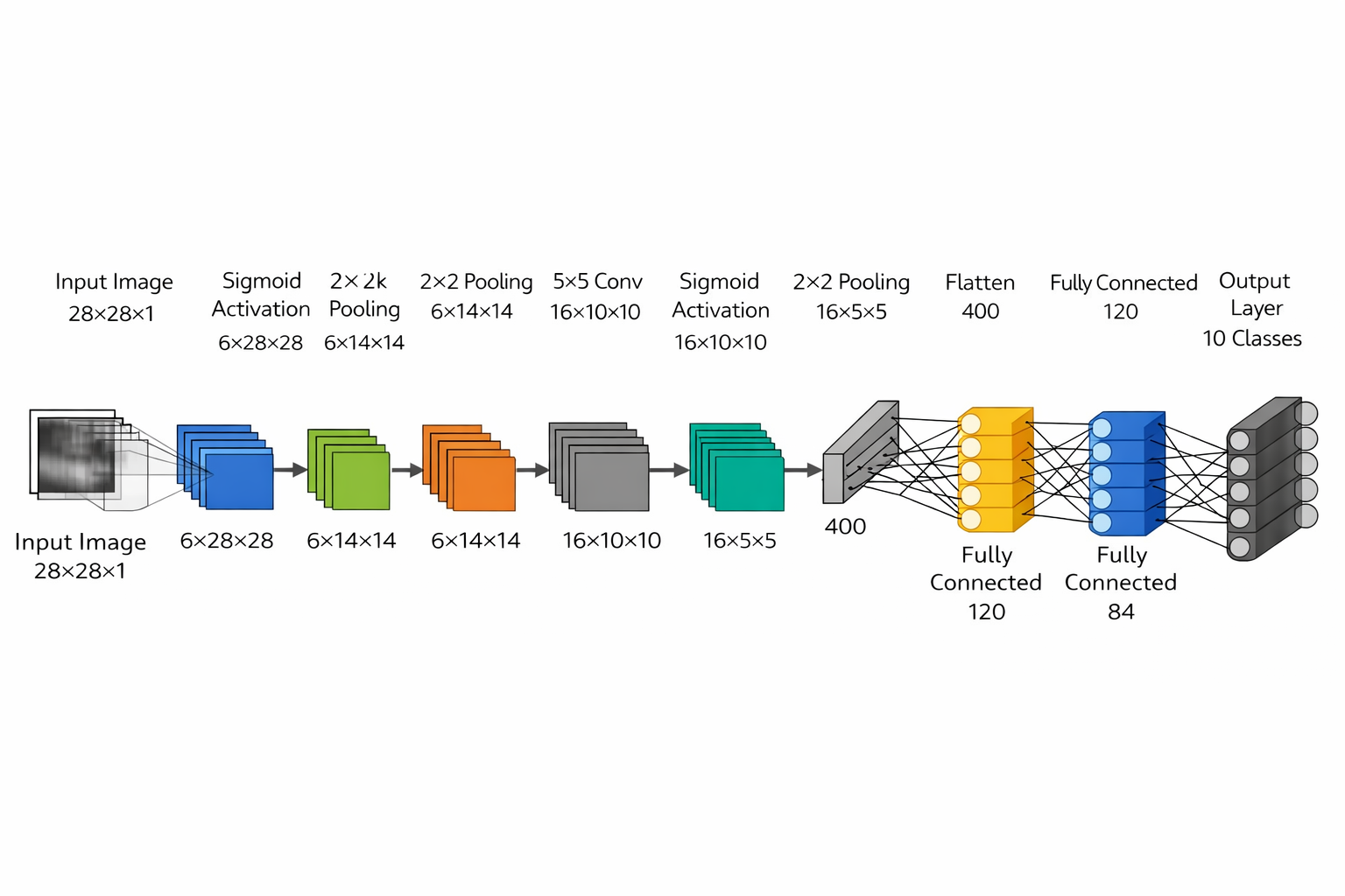
结构流
(1×28×28)
   ↓ Conv
(6×28×28)
   ↓ Pool
(6×14×14)
   ↓ Conv
(16×10×10)
   ↓ Pool
(16×5×5)
   ↓ Flatten
(400)
   ↓ FC
120 → 84 → 10
第一层 卷积
作用:提取最基础特征(边缘/线条)
- 用 6 个卷积核扫描图片
- 每个卷积核学一种“模式”
卷积核一开始是随机初始化的,通过反向传播每个卷积核获得不同梯度,从而逐渐学到不同的特征,实现“自动分工”。
训练结束后的第一层卷积核如下
conv layer 1 kernels shape: (6, 1, 5, 5)
tensor([[[[ 0.4587,  0.9623,  0.8670,  0.4964,  0.3089],
          [ 0.6552,  1.0398,  1.1224,  0.7174,  0.1807],
          [ 0.6282,  1.0901,  1.1454,  0.7885,  0.0931],
          [-0.0701,  0.7881,  0.6510,  0.5285, -0.1383],
          [-0.4480,  0.0050,  0.2505,  0.0305, -0.6273]]],


        [[[ 0.2813, -0.7380, -1.0756,  0.0994,  0.9983],
          [ 0.1324, -1.1169, -1.5388, -0.3630,  0.7220],
          [ 0.5710, -1.2043, -1.3466, -0.2483,  0.9263],
          [ 0.8825, -0.7165, -1.0330, -0.2627,  1.2286],
          [ 0.7197, -0.2831, -0.6991, -0.1023,  1.0881]]],


        [[[-0.2562, -0.3698, -0.5058, -0.5433, -0.2179],
          [-0.2519, -0.9381, -1.3914, -1.2632, -0.6284],
          [-0.1006, -1.0503, -1.5608, -1.2406, -0.6634],
          [-0.0841, -0.8037, -0.9964, -1.0884, -0.1780],
          [ 0.4274, -0.1798, -0.3585, -0.3298,  0.4001]]],


        [[[ 1.3652,  0.3242, -0.6089, -1.1077, -0.3269],
          [ 1.3465,  0.6187, -0.5226, -1.3528, -0.4494],
          [ 1.4649,  0.5162, -0.7658, -1.5320, -0.7495],
          [ 1.3108,  0.6676, -0.6614, -1.3077, -0.4605],
          [ 1.2666,  0.5929, -0.5263, -0.8645, -0.0532]]],


        [[[-0.1916,  0.1918,  0.1830, -0.1576, -0.7518],
          [-0.0383,  0.6332,  0.8412,  0.2415, -0.5478],
          [ 0.0588,  1.0093,  0.8956,  0.5301, -0.4315],
          [-0.2797,  0.6476,  0.5846,  0.3092, -0.4632],
          [-0.4576,  0.3427,  0.4679,  0.0045, -0.7528]]],


        [[[ 0.0822, -0.3571, -1.1740, -1.0378,  0.0807],
          [ 0.0478, -0.9784, -1.6519, -1.5483, -0.4701],
          [ 0.4050, -0.5875, -1.8024, -1.8586, -0.3538],
          [ 0.6129, -0.1174, -1.0187, -1.0747,  0.1752],
          [ 1.0586,  0.1861, -0.2323, -0.1765,  0.5327]]]])
第二层:Sigmoid
作用:加入非线性能力
Sigmoid 的本质作用是引入非线性,把卷积输出映射到 0~1,但由于梯度消失等问题,现代模型已经基本用 ReLU 替代。
第三层:AvgPool2d
作用:降采样 + 抗干扰
本质: “模糊 + 压缩”
- 降低计算量
- 提高鲁棒性
第四层: Conv2d(6 → 16)
作用:组合低级特征 → 高级特征
本质:feature = 边缘的组合
为什么通道变多?
- 特征越来越复杂
- 需要更多“表达能力”
第五层:Sigmoid
作用:加入非线性能力
第六层: AvgPool2d
作用:再次压缩
第七层:Flatten
作用:从“图像”变成“向量”: CNN → MLP 的桥梁
本质:把空间结构:二维 → 一维
第八层:Linear(400 → 120)
作用:特征融合(全局理解)
- 前面是:局部特征
- 这里: 把所有特征组合起来
本质: 分类决策的第一步
第九层:Sigmoid
再次增加非线性
第十层:Linear(120 → 84)
进一步压缩 + 提取更抽象特征
第十一层:Sigmoid
再次增加非线性
第十二层:Linear(84 → 10)
输出 10
作用:分类输出(logits)
每个值代表:属于某一类的“置信度(未归一化)”
神经网络图
参数数量
| 层序号 | 层类型 | 输入尺寸 | 输出尺寸 | 参数计算公式 | 参数量 |
|---|---|---|---|---|---|
| 1 | Conv2d(1→6, 5×5) | 1×28×28 | 6×28×28 | 6×1×5×5 + 6 | 156 |
| 2 | Sigmoid | 6×28×28 | 6×28×28 | 无参数 | 0 |
| 3 | AvgPool2d | 6×28×28 | 6×14×14 | 无参数 | 0 |
| 4 | Conv2d(6→16, 5×5) | 6×14×14 | 16×10×10 | 16×6×5×5 + 16 | 2416 |
| 5 | Sigmoid | 16×10×10 | 16×10×10 | 无参数 | 0 |
| 6 | AvgPool2d | 16×10×10 | 16×5×5 | 无参数 | 0 |
| 7 | Flatten | 16×5×5 | 400 | 无参数 | 0 |
| 8 | Linear(400→120) | 400 | 120 | 120×400 + 120 | 48120 |
| 9 | Sigmoid | 120 | 120 | 无参数 | 0 |
| 10 | Linear(120→84) | 120 | 84 | 84×120 + 84 | 10164 |
| 11 | Sigmoid | 84 | 84 | 无参数 | 0 |
| 12 | Linear(84→10) | 84 | 10 | 10×84 + 10 | 850 |
总计:61,706 参数
这个 LeNet 模型总参数约 6.17 万,其中绝大部分集中在全连接层,这也是现代模型逐渐抛弃 FC 的原因
对比多层感知机的参数数量
| 模型 | 参数量 |
|---|---|
| MLP | ~235K |
| CNN(LeNet) | ~61K |
👉 ✅ 减少了约 75%
0
次点赞