独热编码
# -*- coding: utf-8 -*-
import math
import random
import re
import torch
from torch import nn
from torch.nn import functional as F
from d2l import torch as d2l

# 在 d2l 数据集中注册《时间机器》文本下载地址与校验值
d2l.DATA_HUB['time_machine'] = (d2l.DATA_URL + 'timemachine.txt',
                                '090b5e7e70c295757f55df93cb0a180b9691891a')


def read_time_machine():
    """读取并预处理《时间机器》文本行"""
    # d2l.download 会自动下载并缓存数据文件,返回本地路径
    with open(d2l.download('time_machine'), 'r') as f:
        # lines 是字符串列表,每个元素对应原始文本的一行
        lines = f.readlines()
    # 预处理策略:
    # 1) 非字母字符统一替换为空格
    # 2) 去掉首尾空白
    # 3) 全部转为小写,减少词表稀疏
    return [re.sub('[^A-Za-z]+', ' ', line).strip().lower() for line in lines]


def load_corpus_time_machine(max_tokens=-1):  #@save
    """返回《时间机器》数据集的词元索引序列和词表"""
    # 读取原始文本并清洗
    lines = read_time_machine()
    # 使用字符级分词:每个字符视为一个 token(字符级语言模型常用)
    tokens = d2l.tokenize(lines, 'char')
    # 根据 tokens 构建词表(字符 -> 索引)
    vocab = d2l.Vocab(tokens)
    # 将二维 token 列表展平为一维语料索引序列:
    # [[t,i,m,e], [...], ...] -> [idx_t, idx_i, idx_m, idx_e, ...]
    corpus = [vocab[token] for line in tokens for token in line]
    # 调试时可截断语料长度,加快实验速度
    if max_tokens > 0:
        corpus = corpus[:max_tokens]
    return corpus, vocab


def seq_data_iter_random(corpus, batch_size, num_steps):  #@save
    """使用随机抽样生成一个小批量子序列"""
    # 随机偏移起点,避免每次都从同一位置切分
    corpus = corpus[random.randint(0, num_steps - 1):]
    # 可切出的子序列个数(每段长度为 num_steps)
    num_subseqs = (len(corpus) - 1) // num_steps
    # 每段子序列的起始索引:0, num_steps, 2*num_steps, ...
    initial_indices = list(range(0, num_subseqs * num_steps, num_steps))
    # 打乱子序列起点,实现随机采样
    random.shuffle(initial_indices)

    def data(pos):
        # 取出从 pos 开始、长度为 num_steps 的片段
        return corpus[pos: pos + num_steps]

    # 可形成的小批量数
    num_batches = num_subseqs // batch_size
    for i in range(0, batch_size * num_batches, batch_size):
        # 当前批次选 batch_size 个起点
        initial_indices_per_batch = initial_indices[i: i + batch_size]
        # X 是输入片段,Y 是右移一位后的标签片段
        X = [data(j) for j in initial_indices_per_batch]
        Y = [data(j + 1) for j in initial_indices_per_batch]
        # 输出形状:(batch_size, num_steps)
        yield torch.tensor(X), torch.tensor(Y)


def seq_data_iter_sequential(corpus, batch_size, num_steps):  #@save
    """使用顺序分区生成一个小批量子序列"""
    # 顺序分区也做一个随机偏移,降低固定切分带来的偏置
    offset = random.randint(0, num_steps)
    # 令 token 总数可被 batch_size 整除,便于 reshape
    num_tokens = ((len(corpus) - offset - 1) // batch_size) * batch_size
    # X 是原序列片段,Y 是整体右移一位的片段
    Xs = torch.tensor(corpus[offset: offset + num_tokens])
    Ys = torch.tensor(corpus[offset + 1: offset + 1 + num_tokens])
    # 按 batch 维重排:每行是一条连续子序列
    Xs, Ys = Xs.reshape(batch_size, -1), Ys.reshape(batch_size, -1)
    # 沿时间维切成多个长度为 num_steps 的小块
    num_batches = Xs.shape[1] // num_steps
    for i in range(0, num_steps * num_batches, num_steps):
        X = Xs[:, i: i + num_steps]
        Y = Ys[:, i: i + num_steps]
        yield X, Y


class SeqDataLoader:  #@save
    """加载序列数据的迭代器"""
    def __init__(self, batch_size, num_steps, use_random_iter, max_tokens):
        # 1) 选择子序列采样函数(随机采样 or 顺序分区)
        if use_random_iter:
            self.data_iter_fn = seq_data_iter_random
        else:
            self.data_iter_fn = seq_data_iter_sequential
        # 2) 加载语料索引序列与词表
        self.corpus, self.vocab = load_corpus_time_machine(max_tokens)
        # 3) 保存批量大小与时间步长度配置
        self.batch_size, self.num_steps = batch_size, num_steps

    def __iter__(self):
        # 返回一个生成器;每次迭代产出 (X, Y)
        return self.data_iter_fn(self.corpus, self.batch_size, self.num_steps)

def load_data_time_machine(batch_size, num_steps,  #@save
                           use_random_iter=False, max_tokens=10000):
    """返回时光机器数据集的迭代器和词表"""
    # 封装统一数据加载入口:便于后续模型代码直接调用
    data_iter = SeqDataLoader(
        batch_size, num_steps, use_random_iter, max_tokens)
    return data_iter, data_iter.vocab

# batch_size:每个小批量的样本数
# num_steps:RNN 每次展开的时间步数(序列长度)
batch_size, num_steps = 32, 35
# 加载《时间机器》数据集:
# train_iter 为训练迭代器,vocab 为词表对象
train_iter, vocab = load_data_time_machine(batch_size, num_steps)

# 构造一个形状为 (batch_size=2, num_steps=5) 的整数索引矩阵
# 每一行可以理解为一个样本序列
X = torch.arange(10).reshape((2, 5))

# 打印关键信息,直观看独热编码前后变化
print("原始索引矩阵 X:")
print(X)
print("转置后的 X.T(时间步在前):")
print(X.T)

Y = F.one_hot(X.T, 28)
print("独热编码后张量 Y 的形状:", Y.shape)
print("说明:形状含义为 (时间步数, batch_size, 词表大小)")
print("整个输入数据的独热编码张量 Y:")
print(Y)
运行结果
原始索引矩阵 X:
tensor([[0, 1, 2, 3, 4],
        [5, 6, 7, 8, 9]])
转置后的 X.T(时间步在前):
tensor([[0, 5],
        [1, 6],
        [2, 7],
        [3, 8],
        [4, 9]])
独热编码后张量 Y 的形状: torch.Size([5, 2, 28])
说明:形状含义为 (时间步数, batch_size, 词表大小)
整个输入数据的独热编码张量 Y:
tensor([[[1, 0, 0, 0, 0, 0, 0, 0, 0, 0, 0, 0, 0, 0, 0, 0, 0, 0, 0, 0, 0, 0, 0,
          0, 0, 0, 0, 0],
         [0, 0, 0, 0, 0, 1, 0, 0, 0, 0, 0, 0, 0, 0, 0, 0, 0, 0, 0, 0, 0, 0, 0,
          0, 0, 0, 0, 0]],

        [[0, 1, 0, 0, 0, 0, 0, 0, 0, 0, 0, 0, 0, 0, 0, 0, 0, 0, 0, 0, 0, 0, 0,
          0, 0, 0, 0, 0],
         [0, 0, 0, 0, 0, 0, 1, 0, 0, 0, 0, 0, 0, 0, 0, 0, 0, 0, 0, 0, 0, 0, 0,
          0, 0, 0, 0, 0]],

        [[0, 0, 1, 0, 0, 0, 0, 0, 0, 0, 0, 0, 0, 0, 0, 0, 0, 0, 0, 0, 0, 0, 0,
          0, 0, 0, 0, 0],
         [0, 0, 0, 0, 0, 0, 0, 1, 0, 0, 0, 0, 0, 0, 0, 0, 0, 0, 0, 0, 0, 0, 0,
          0, 0, 0, 0, 0]],

        [[0, 0, 0, 1, 0, 0, 0, 0, 0, 0, 0, 0, 0, 0, 0, 0, 0, 0, 0, 0, 0, 0, 0,
          0, 0, 0, 0, 0],
         [0, 0, 0, 0, 0, 0, 0, 0, 1, 0, 0, 0, 0, 0, 0, 0, 0, 0, 0, 0, 0, 0, 0,
          0, 0, 0, 0, 0]],

        [[0, 0, 0, 0, 1, 0, 0, 0, 0, 0, 0, 0, 0, 0, 0, 0, 0, 0, 0, 0, 0, 0, 0,
          0, 0, 0, 0, 0],
         [0, 0, 0, 0, 0, 0, 0, 0, 0, 1, 0, 0, 0, 0, 0, 0, 0, 0, 0, 0, 0, 0, 0,
          0, 0, 0, 0, 0]]])
Step 1:构造输入 X
原始数据
X =
[[0, 1, 2, 3, 4],
 [5, 6, 7, 8, 9]]
| 维度 | 含义 |
|---|---|
| 2 | batch_size(两条序列) |
| 5 | num_steps(每条序列长度) |
Step 2:RNN视角
X.T 转置

[[0, 5],
 [1, 6],
 [2, 7],
 [3, 8],
 [4, 9]]
(2, 5) → (5, 2)
| 维度 | 含义 |
|---|---|
| 5 | 时间步 |
| 2 | batch |
RNN不是按“句子”处理,而是按“时间步”处理
t=0: [0, 5]
t=1: [1, 6]
t=2: [2, 7]
t=3: [3, 8]
t=4: [4, 9]
每一个时间步,同时喂 batch 里的所有样本
Step 3:one-hot 编码
Y = F.one_hot(X.T, 28)

Y.shape = (5, 2, 28)
| 维度 | 含义 |
|---|---|
| 5 | 时间步 |
| 2 | batch |
| 28 | 词表大小 |
完整流程
Step1: 原始数据
X = (batch, time)

        ↓

Step2: 转置
X.T = (time, batch)

        ↓

Step3: one-hot
Y = (time, batch, vocab)

        ↓

Step4: RNN逐步读取
Xt = (batch, vocab)
类比理解
想象你在看 2 部电影(batch=2)
每部电影 5 帧(time=5):
电影1: 0 1 2 3 4
电影2: 5 6 7 8 9
RNN的看法是:
第1帧:同时看两部电影 → [0,5]
第2帧:同时看 → [1,6]
第3帧:同时看 → [2,7]
...
然后每一帧都变成:one-hot图像(特征向量)
理论基础
生成答案
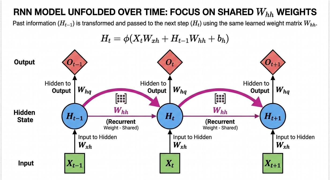
完整的 RNN 逻辑由两个公式组成:
动作一:更新记忆(你看到的公式)
\[H_t = \phi(X_t W_{xh} + H_{t-1} W_{hh} + b_h)\]动作二:生成输出(答案就在这里)
\[O_t = H_t W_{hq} + b_q\]在一个标准的单层 RNN 中,训练最终是为了得到以下 5 个关键参数:
- 负责“处理当前”的权重:$W_{xh}$
- 负责“连接过去”的权重:$W_{hh}$
- 负责“提取答案”的权重:$W_{hq}$
- $b_h$:隐藏层的偏置,调节记忆生成的灵敏度。
- $b_q$:输出层的偏置,调节最终预测值的基准线。
| 参数 | 职责 | 更准确的类比 |
|---|---|---|
| Wxh | 处理当前输入 | 👀 观察力(怎么看新信息) |
| Whh | 处理过去记忆 | 🧠 理解/联想力(怎么解读已有印象) |
| Whq | 生成输出 | 🗣️ 表达力(怎么说出来) |
| bh, bq | 偏置调整 | 🎯 默认倾向 / 直觉偏好 |
初始化模型参数
def get_params(vocab_size, num_hiddens, device):
    num_inputs = num_outputs = vocab_size

    def normal(shape):
        return torch.randn(size=shape, device=device) * 0.01

    # 隐藏层参数
    # 负责“处理当前”的权重
    W_xh = normal((num_inputs, num_hiddens))
    # 负责“连接过去”的权重
    W_hh = normal((num_hiddens, num_hiddens))
    # 隐藏层偏置项
    b_h = torch.zeros(num_hiddens, device=device)
    # 负责“提取答案”的权重
    W_hq = normal((num_hiddens, num_outputs))
    # 输出层偏置项
    b_q = torch.zeros(num_outputs, device=device)
    # 附加梯度
    params = [W_xh, W_hh, b_h, W_hq, b_q]
    for param in params:
        param.requires_grad_(True)
    return params
各个参数的位置结构图
          当前输入 X_t
                │
                ▼
          [ W_xh ]
                │
                ▼
           (当前特征)
                │
                ├──────────────┐
                │              │
                ▼              ▼
        上一状态 H_{t-1}   [ W_hh ]
                │              │
                ▼              ▼
           (历史信息)──────────┘
                │
                ▼
           + b_h
                │
                ▼
             tanh
                │
                ▼
              H_t
                │
                ▼
           [ W_hq ]
                │
                ▼
              Y_t
循环神经网络模型
def init_rnn_state(batch_size, num_hiddens, device):
    # RNN 初始隐藏状态 H_0:全零张量
    # 返回元组是为了兼容可能含多个状态的模型(如 LSTM 有 H 和 C)
    return (torch.zeros((batch_size, num_hiddens), device=device), )

def rnn(inputs, state, params):
    # inputs的形状:(时间步数量,批量大小,词表大小)
    W_xh, W_hh, b_h, W_hq, b_q = params
    # 当前隐藏状态,形状:(batch_size, num_hiddens)
    H, = state
    # 收集每个时间步的输出
    outputs = []
    # X的形状:(批量大小,词表大小)
    for X in inputs:
        # 经典 RNN 状态更新公式:
        # H_t = tanh(X_t W_xh + H_{t-1} W_hh + b_h)
        H = torch.tanh(torch.mm(X, W_xh) + torch.mm(H, W_hh) + b_h)
        # 输出层(未过 softmax,保留 logits 供后续交叉熵使用)
        Y = torch.mm(H, W_hq) + b_q
        outputs.append(Y)
    # 沿时间维拼接输出:
    # 原本是 num_steps 个 (batch_size, vocab_size)
    # 拼接后为 (num_steps * batch_size, vocab_size)
    return torch.cat(outputs, dim=0), (H,)

class RNNModelScratch: #@save
    """从零开始实现的循环神经网络模型"""
    def __init__(self, vocab_size, num_hiddens, device,
                 get_params, init_state, forward_fn):
        # 保存超参数与函数句柄
        self.vocab_size, self.num_hiddens = vocab_size, num_hiddens
        # 初始化可训练参数
        self.params = get_params(vocab_size, num_hiddens, device)
        # 保存状态初始化函数与前向计算函数
        self.init_state, self.forward_fn = init_state, forward_fn

    def __call__(self, X, state):
        # 输入 X 形状:(batch_size, num_steps)
        # 转换为 one-hot 并转置为时间步优先:
        # (num_steps, batch_size, vocab_size)
        X = F.one_hot(X.T, self.vocab_size).type(torch.float32)
        return self.forward_fn(X, state, self.params)

    def begin_state(self, batch_size, device):
        # 按当前 batch 大小创建初始隐藏状态
        return self.init_state(batch_size, self.num_hiddens, device)

# 隐藏单元数量(决定模型容量)
num_hiddens = 512
# 实例化从零实现的 RNN 模型
device = d2l.try_gpu()
net = RNNModelScratch(len(vocab), num_hiddens, device, get_params,
                      init_rnn_state, rnn)

# 打印模型结构关键信息,帮助理解“从零实现”的 RNN 由哪些部分组成
print("\n===== RNNModelScratch 结构信息 =====")
print(f"设备: {device}")
print(f"词表大小(vocab_size): {net.vocab_size}")
print(f"隐藏单元数(num_hiddens): {net.num_hiddens}")
param_names = ["W_xh(输入->隐藏)", "W_hh(隐藏->隐藏)", "b_h(隐藏偏置)",
               "W_hq(隐藏->输出)", "b_q(输出偏置)"]
total_params = 0
for name, param in zip(param_names, net.params):
    total_params += param.numel()
    print(f"{name} 形状: {tuple(param.shape)}, 参数量: {param.numel()}")
print(f"参数总量: {total_params}")

# 创建初始状态并做一次前向传播,检查输出维度是否正确
state = net.begin_state(X.shape[0], device)
Y, new_state = net(X.to(device), state)
# Y.shape: (num_steps * batch_size, vocab_size)
# len(new_state): 状态元组长度(RNN 为 1)
# new_state[0].shape: (batch_size, num_hiddens)
print("\n===== 一次前向传播的张量形状 =====")
print(f"输入 X 形状: {tuple(X.shape)}")
print(f"初始隐藏状态 state[0] 形状: {tuple(state[0].shape)}")
print(f"输出 Y 形状: {tuple(Y.shape)}")
print(f"新隐藏状态数量: {len(new_state)}")
print(f"新隐藏状态 new_state[0] 形状: {tuple(new_state[0].shape)}")
运行结果
==== RNNModelScratch 结构信息 =====
设备: cuda:0
词表大小(vocab_size): 28
隐藏单元数(num_hiddens): 512
W_xh(输入->隐藏) 形状: (28, 512), 参数量: 14336
W_hh(隐藏->隐藏) 形状: (512, 512), 参数量: 262144
b_h(隐藏偏置) 形状: (512,), 参数量: 512
W_hq(隐藏->输出) 形状: (512, 28), 参数量: 14336
b_q(输出偏置) 形状: (28,), 参数量: 28
参数总量: 291356

===== 一次前向传播的张量形状 =====
输入 X 形状: (2, 5)
初始隐藏状态 state[0] 形状: (2, 512)
输出 Y 形状: (10, 28)
新隐藏状态数量: 1
新隐藏状态 new_state[0] 形状: (2, 512)
整体调用链
输入 X (batch, time)
        │
        ▼
转置 + one-hot
        │
        ▼
(time, batch, vocab)
        │
        ▼
for t in time:
    │
    ├── X_t (batch, vocab)
    │
    ├── H = tanh(XW + HW)
    │
    ├── Y_t = H W_hq
    │
    └── 保存输出
        │
        ▼
拼接 outputs
        │
        ▼
(time * batch, vocab)
三个关键理解
- RNN 一时间步一时间步处理
- H只是中间变量,模型的“记忆核心”
- 每个时间步都有输出
预测
def predict_ch8(prefix, num_preds, net, vocab, device):  #@save
    """在prefix后面生成新字符"""
    # 推理阶段 batch_size 固定为 1:一次只生成一条序列
    state = net.begin_state(batch_size=1, device=device)
    # outputs 保存“已生成/已喂入”的词元索引,先放入前缀首字符
    outputs = [vocab[prefix[0]]]
    # 每次仅把“上一个词元”作为当前输入,形状保持为 (1, 1)
    # 其中:
    # - 第 1 维是 batch 维(batch_size=1)
    # - 第 2 维是时间步维(num_steps=1)
    get_input = lambda: torch.tensor([outputs[-1]], device=device).reshape((1, 1))
    # 预热期(warm-up):
    # 用 prefix 的后续字符逐步更新隐藏状态,让模型“进入上下文”
    # 注意:预热期不依赖模型预测结果,而是喂入真实前缀字符
    for y in prefix[1:]:
        _, state = net(get_input(), state)
        outputs.append(vocab[y])

    # 自回归生成阶段:
    # 每一步都基于“上一步输出词元”继续预测下一个词元
    for _ in range(num_preds):
        y, state = net(get_input(), state)
        # y 形状约为 (1, vocab_size),表示下一个字符的打分(logits)
        # 这里使用贪心策略:取分数最大的词元索引作为当前步输出
        outputs.append(int(y.argmax(dim=1).reshape(1)))

    # 将索引序列映射回字符并拼接成字符串
    return ''.join([vocab.idx_to_token[i] for i in outputs])

# 示例:给定前缀 "time traveller ",继续生成 10 个字符
print(predict_ch8('time traveller ', 10, net, vocab, d2l.try_gpu()))
流程图
prefix: "time traveller "

        │
        ▼
【预热阶段】
逐字符喂入 → 更新隐藏状态H

        │
        ▼
【预测阶段】
用最后状态 → 预测下一个字符
        │
        ▼
把预测结果再喂回去(自回归)
阶段一:预热(Warm-up)
让RNN“进入语境”
阶段二:正式预测
一边生成,一边吃自己生成的结果
一次只喂一个字符
完整数据流
初始:
H = 0

【预热阶段】
t → H1
i → H2
m → H3
e → H4

【预测阶段】
H4 → 预测 ' '
' ' → H5 → 预测 't'
't' → H6 → 预测 'r'
...
| 阶段 | 输入 |
|---|---|
| 训练 | 一整个序列 |
| 推理 | 一个一个喂 |
梯度裁剪
def grad_clipping(net, theta):  #@save
    """裁剪梯度"""
    if isinstance(net, nn.Module):
        params = [p for p in net.parameters() if p.requires_grad]
    else:
        params = net.params
    norm = torch.sqrt(sum(torch.sum((p.grad ** 2)) for p in params))
    if norm > theta:
        for param in params:
            param.grad[:] *= theta / norm
理解“RNN 的梯度”,本质就是理解:信息和误差如何在“时间上流动”
❌ 不需要为每个时间步保存一份“参数” ✅ 只需要一份参数,但要保留每个时间步的“中间状态”用于反向传播
👉 RNN 是“参数共享”的网络
那到底“要保存什么”?
✅ 每个时间步的隐藏状态 H_t(以及中间计算图)
RNN 如何解决梯度爆炸和消失问题
问题本质
梯度 ≈ W_hh × W_hh × W_hh × …
结果只有三种:
| 情况 | 结果 |
|---|---|
| >1 | 💥 爆炸 |
| <1 | ❄️ 消失 |
| ≈1 | ✅ 稳定 |
“止血类”(缓解问题)
| 方法 | 解决什么 | 优点 | ❌ 缺点 |
|---|---|---|---|
| 梯度裁剪 | 梯度爆炸 | 简单、通用、几乎零成本 | ❗只能防爆炸,无法解决梯度消失;过强会影响收敛速度 |
| 截断 BPTT | 爆炸 + 内存 | 降低计算量,训练稳定 | ❗丢失长期依赖(只能学短期模式) |
| 正则化(L2/Dropout) | 稳定训练 | 防过拟合,提高泛化 | ❗对梯度问题是间接作用,效果有限;Dropout在RNN中不好用(需要特殊变种) |
“结构类”(根本改造)
| 方法 | 核心思想 | 优点 | ❌ 缺点 |
|---|---|---|---|
| LSTM | 梯度≈1传递(加法路径 + 门控) | ✅ 能学长期依赖 ✅ 训练稳定 |
❗结构复杂(参数多) ❗计算慢 |
| GRU | 简化版LSTM | ✅ 参数更少 ✅ 收敛更快 |
❗表达能力略弱(某些复杂任务不如LSTM) |
| 残差RNN | 加直连路径(类似ResNet) | ✅ 缓解梯度消失 ✅ 易训练 |
❗提升有限 ❗不如LSTM稳定 |
| Transformer | 去掉循环,用Attention | ✅ 无梯度消失(无时间连乘) ✅ 并行计算快 |
❗显存消耗大(O(n²)) ❗对长序列成本高 |
👉 RNN的问题本质是“时间上的连乘不稳定”,所有优化方法本质都是在“避免连乘”
训练
#@save
def train_epoch_ch8(net, train_iter, loss, updater, device, use_random_iter):
"""训练网络一个迭代周期(定义见第8章)"""
# state: RNN 的隐藏状态(跨小批量复用)
# timer: 统计本轮训练耗时,用于计算吞吐率(词元/秒)
state, timer = None, d2l.Timer()
# metric[0]: 累计损失(按词元数量加权)
# metric[1]: 累计词元数
metric = d2l.Accumulator(2) # 训练损失之和,词元数量
for X, Y in train_iter:
if state is None or use_random_iter:
# 在第一次迭代或使用随机抽样时初始化state
# 随机抽样时,不同批次的片段通常不连续,不能沿用上一批状态
state = net.begin_state(batch_size=X.shape[0], device=device)
else:
if isinstance(net, nn.Module) and not isinstance(state, tuple):
# state对于nn.GRU是个张量
# 与计算图断开,避免反向传播跨越整个历史序列
state.detach_()
else:
# state对于nn.LSTM或对于我们从零开始实现的模型是个张量
# 元组中每个状态都要 detach,执行截断反向传播(TBPTT)
for s in state:
s.detach_()
# 标签 Y 原始形状为 (batch_size, num_steps)
# 转置后展平为一维,和 y_hat 的前两维展平结果对齐
y = Y.T.reshape(-1)
# 将数据搬到训练设备(CPU/GPU)
X, y = X.to(device), y.to(device)
# 前向传播:
# y_hat 形状通常为 (batch_size*num_steps, vocab_size)
# state 为当前批次结束后的隐藏状态
y_hat, state = net(X, state)
# 交叉熵默认按样本求平均,这里取 mean 得到标量 loss
l = loss(y_hat, y.long()).mean()
if isinstance(updater, torch.optim.Optimizer):
# 使用 PyTorch 优化器的标准三步:清梯度 -> 反传 -> 参数更新
updater.zero_grad()
l.backward()
# 反传后先做梯度裁剪,再执行 step,降低梯度爆炸风险
grad_clipping(net, 1)
updater.step()
else:
# 从零实现分支:手工反向传播 + 手工参数更新
l.backward()
grad_clipping(net, 1)
# 因为已经调用了mean函数
updater(batch_size=1)
# 将“平均损失”还原成“总损失”再累计,便于跨批次准确求平均
metric.add(l * y.numel(), y.numel())
# 返回:
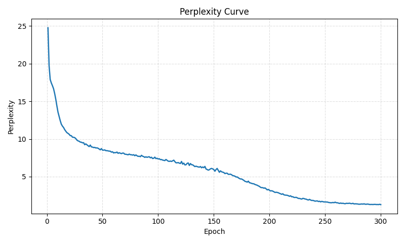
# 1) 困惑度 perplexity = exp(平均交叉熵)
# 2) 训练速度 = 总词元数 / 总耗时
return math.exp(metric[0] / metric[1]), metric[1] / timer.stop()
#@save
def train_ch8(net, train_iter, vocab, lr, num_epochs, device,
use_random_iter=False, plot=False):
"""训练模型(定义见第8章)"""
# 字符级语言模型是多分类任务,目标是预测“下一个字符”
loss = nn.CrossEntropyLoss()
animator = None
if plot:
# 可选可视化:横轴 epoch,纵轴困惑度
animator = d2l.Animator(xlabel='epoch', ylabel='perplexity',
legend=['train'], xlim=[10, num_epochs])
# 初始化
if isinstance(net, nn.Module):
# 若是高级 API 模型,直接使用 SGD 优化器
updater = torch.optim.SGD(net.parameters(), lr)
else:
# 从零实现模型使用 d2l.sgd 手工更新参数
updater = lambda batch_size: d2l.sgd(net.params, lr, batch_size)
# 固定一个“前缀到续写”的预测函数,便于训练中观察生成质量
predict = lambda prefix: predict_ch8(prefix, 50, net, vocab, device)
# 训练和预测
for epoch in range(num_epochs):
# 每个 epoch 调用一次“单轮训练”并返回本轮困惑度与速度
ppl, speed = train_epoch_ch8(
net, train_iter, loss, updater, device, use_random_iter)
if (epoch + 1) % 10 == 0:
# 每 10 轮打印一次训练指标与示例文本,便于观察收敛趋势
print(f'epoch {epoch + 1:>3d}, 困惑度 {ppl:.2f}, 速度 {speed:.1f} 词元/秒')
print(predict('time traveller'))
if animator is not None:
animator.add(epoch + 1, [ppl])
# 训练结束后输出最终指标与两条续写示例
print(f'困惑度 {ppl:.1f}, {speed:.1f} 词元/秒 {str(device)}')
print(predict('time traveller'))
print(predict('traveller'))
# 训练总轮数与学习率:
# - num_epochs 越大通常越容易收敛,但训练更耗时
# - lr 过大可能震荡,过小会收敛慢
num_epochs, lr = 200, 1
train_ch8(net, train_iter, vocab, lr, num_epochs, device, plot=False)
运行结果
time traveller m<unk>d<unk>ofotpb
epoch  10, 困惑度 13.60, 速度 94993.1 词元/秒
time traveller the the the the the the the the the the the the t
epoch  20, 困惑度 10.60, 速度 105968.7 词元/秒
time travellere the the the the the the the the the the the the
epoch  30, 困惑度 9.47, 速度 94884.4 词元/秒
time traveller the the the the the the the the the the the the t
epoch  40, 困惑度 9.02, 速度 92587.7 词元/秒
time travellere the the the the the the the the the the the the
epoch  50, 困惑度 8.59, 速度 101066.2 词元/秒
time traveller and the the the the the the the the the the the t
epoch  60, 困惑度 8.24, 速度 94710.3 词元/秒
time traveller and the the thing the the thing the the thing the
epoch  70, 困惑度 7.99, 速度 94960.4 词元/秒
time traveller and the the this the this the this the this the t
epoch  80, 困惑度 7.77, 速度 94281.0 词元/秒
time travellere the the the the the the the the the the the the
epoch  90, 困惑度 7.61, 速度 108433.1 词元/秒
time traveller the the the the the the the the the the the the t
epoch 100, 困惑度 7.51, 速度 95367.7 词元/秒
time travellere the in the paree thay ur and he paree thay ur an
epoch 110, 困惑度 7.18, 速度 98329.3 词元/秒
time traveller and the the the the the the the the the the the t
epoch 120, 困惑度 6.94, 速度 95804.6 词元/秒
time traveller the this the thime thave in the this the thime th
epoch 130, 困惑度 6.65, 速度 118833.5 词元/秒
time traveller ace arimethere and have and the pereat in the med
epoch 140, 困惑度 6.24, 速度 115627.3 词元/秒
time traveller arly the that heat in the that there and the tine
epoch 150, 困惑度 5.85, 速度 118396.9 词元/秒
time traveller of the that there than ther time traveller of the
epoch 160, 困惑度 5.57, 速度 118132.3 词元/秒
time travelleris the grace asmere the that is allarthot it tome
epoch 170, 困惑度 4.88, 速度 117554.8 词元/秒
time traveller of chate an thit is so the fice travel the tion a
epoch 180, 困惑度 4.24, 速度 117874.4 词元/秒
time travellerit t and him thane dimensions a tonthe thrye what
epoch 190, 困惑度 3.62, 速度 116736.8 词元/秒
time traveller as ingh wertime sour a dinels mevere curnow ta th
epoch 200, 困惑度 3.19, 速度 117819.7 词元/秒
time traveller thic odiches of cout in this sous atwir asceriled
epoch 210, 困惑度 2.76, 速度 117646.8 词元/秒
time traveller tho ghas sthe wird oc a simelt are ie the this sa
epoch 220, 困惑度 2.32, 速度 117847.5 词元/秒
time traveller trientan e is thes but instancidif caref in the m
epoch 230, 困惑度 2.00, 速度 115389.8 词元/秒
time traveller asting has expand wither aime sime soing inst of
epoch 240, 困惑度 1.79, 速度 117774.3 词元/秒
time traveller arover therentthen shint alwhat heand treestom th
epoch 250, 困惑度 1.67, 速度 117088.9 词元/秒
time traveller ast athing now in whr hit sact motting breinot br
epoch 260, 困惑度 1.51, 速度 117543.4 词元/秒
time traveller arthat brechas the oome hap asatheplonen to ee th
epoch 270, 困惑度 1.42, 速度 117500.4 词元/秒
time traveller thoughand was acoully s only two dementions of sp
epoch 280, 困惑度 1.37, 速度 113864.5 词元/秒
time travellerit to gaint ureat ais all in the grome sishe long
epoch 290, 困惑度 1.33, 速度 117508.4 词元/秒
time traveller herd and the time travellerit would be remarkably
epoch 300, 困惑度 1.31, 速度 115886.5 词元/秒
time traveller ablent hibhe dinstift is coreresthat it yom verag
困惑度 1.3, 115886.5 词元/秒 cuda:0
time traveller ablent hibhe dinstift is coreresthat it yom verag
travellerractlyus io cime ssuelly tome aime for somattime a
理解
一条长序列
↓
被切成很多 batch(时间片)
↓
每个 batch 做“局部时间反传”
↓
通过 state 串起来


当前 batch 的起点 = 上一个 batch 的终点

... → batch1 → batch2 → batch3 ...
detach
👉 人为截断时间反传(TBPTT)
state.detach_()

👉 这一行的本质:

👉 切断梯度,但不切断数值

🧠 用一句话解释:
状态传递 ✔
梯度不传 ❌
为什么必须这样?
如果不 detach:

batch1 → batch2 → batch3 → batch4 → ...

👉 梯度会变成:

从 batchN 一直回到最开始

👉 结果:

❌ 显存爆炸
❌ 梯度爆炸
❌ 训练不可控
困惑度
| 阶段 | 困惑度 | 模型状态 |
|---|---|---|
| 初期 | 10+ | 完全不会 |
| 中期 | 5~8 | 学会词频 |
| 后期 | 2~4 | 学会短句 |
| 现在 | ≈1 | ❗几乎在“背书” |
困惑度的计算
metric[0] = 总损失(交叉熵累计)
metric[1] = 总token数

→ 平均损失 = metric[0] / metric[1]

→ perplexity = exp(平均损失)
循环神经网络的简洁实现
import torch
from torch import nn
from torch.nn import functional as F
from d2l import torch as d2l
import my_d2l

# ---------------------------
# 1) 数据加载
# ---------------------------
# batch_size: 每个小批量包含多少条序列
# num_steps: 每条序列的时间步长度(RNN 展开长度)
batch_size, num_steps = 32, 35
# 读取“时间机器”字符级数据集:
# train_iter 会按 (X, Y) 迭代小批量数据
# vocab 为字符词表(字符 <-> 索引)
train_iter, vocab = my_d2l.load_data_time_machine(batch_size, num_steps)

# ---------------------------
# 2) 先直接使用 nn.RNN 看输入输出形状
# ---------------------------
# 隐藏单元数(hidden size)决定 RNN 的状态表示能力
num_hiddens = 256
# 输入维度=input_size=词表大小(因为后面用 one-hot 作为输入)
# 输出维度=hidden_size=num_hiddens
rnn_layer = nn.RNN(len(vocab), num_hiddens)

# 手动构造初始隐藏状态 h0:
# 形状=(num_layers * num_directions, batch_size, hidden_size)
# 这里是单层单向 RNN,所以第一维为 1
state = torch.zeros((1, batch_size, num_hiddens))
print("隐藏层数,批量大小,隐藏单元数:", state.shape)

#@save
class RNNModel(nn.Module):
    """循环神经网络模型"""
    def __init__(self, rnn_layer, vocab_size, **kwargs):
        super(RNNModel, self).__init__(**kwargs)
        # 底层循环层(可替换为 nn.RNN/nn.GRU/nn.LSTM)
        self.rnn = rnn_layer
        # 词表大小,用于 one-hot 编码和输出层类别数
        self.vocab_size = vocab_size
        # 隐藏状态维度(hidden_size)
        self.num_hiddens = self.rnn.hidden_size
        # 如果RNN是双向的(之后将介绍),num_directions应该是2,否则应该是1
        if not self.rnn.bidirectional:
            self.num_directions = 1
            # 单向 RNN:每个时间步输出维度为 num_hiddens
            # 线性层将其映射到 vocab_size,得到每个字符类别的 logits
            self.linear = nn.Linear(self.num_hiddens, self.vocab_size)
        else:
            self.num_directions = 2
            # 双向 RNN:每个时间步输出维度变为 2*num_hiddens
            self.linear = nn.Linear(self.num_hiddens * 2, self.vocab_size)

    def forward(self, inputs, state):
        # inputs 原始形状:(batch_size, num_steps)
        # 转置后变为:(num_steps, batch_size)
        # 再做 one-hot,得到:(num_steps, batch_size, vocab_size)
        X = F.one_hot(inputs.T.long(), self.vocab_size)
        # RNN 接受浮点输入
        X = X.to(torch.float32)
        # Y: 每个时间步的隐藏输出
        # state: 最后一个时间步的隐藏状态(或 LSTM 的 (h, c))
        Y, state = self.rnn(X, state)
        # 全连接层首先将Y的形状改为(时间步数*批量大小,隐藏单元数)
        # 它的输出形状是(时间步数*批量大小,词表大小)。
        output = self.linear(Y.reshape((-1, Y.shape[-1])))
        return output, state

    def begin_state(self, device, batch_size=1):
        # 统一创建“与当前网络结构匹配”的初始隐藏状态
        # 第一维始终是 num_layers * num_directions
        if not isinstance(self.rnn, nn.LSTM):
            # nn.GRU以张量作为隐状态
            return  torch.zeros((self.num_directions * self.rnn.num_layers,
                                 batch_size, self.num_hiddens),
                                device=device)
        else:
            # nn.LSTM以元组作为隐状态
            # 返回 (h0, c0),两个张量形状相同
            return (torch.zeros((
                self.num_directions * self.rnn.num_layers,
                batch_size, self.num_hiddens), device=device),
                    torch.zeros((
                        self.num_directions * self.rnn.num_layers,
                        batch_size, self.num_hiddens), device=device))

# ---------------------------
# 3) 模型实例化与简单预测
# ---------------------------
device = d2l.try_gpu()
# 将“底层 rnn_layer + 输出线性层”封装为完整语言模型
net = RNNModel(rnn_layer, vocab_size=len(vocab))
# 移动到训练设备(GPU/CPU)
net = net.to(device)
# 训练前先做一次续写测试,观察随机初始化模型的输出
print(predict_ch8('time traveller', 10, net, vocab, device))

# ---------------------------
# 4) 训练
# ---------------------------
# num_epochs: 训练轮数
# lr: 学习率(对 RNN 从零/简洁实现,d2l 常用 1)
num_epochs, lr = 500, 1
# d2l.train_ch8 会完成:
# - 按 epoch 训练
# - 计算并打印困惑度
# - 定期输出生成文本示例
d2l.train_ch8(net, train_iter, vocab, lr, num_epochs, device)
| 内容 | 手写版 | nn.RNN |
|---|---|---|
| 权重 | 自己定义 | 自动创建 |
| 前向传播 | 手写循环 | C++优化 |
| 反向传播 | autograd | autograd |
| 多层RNN | 要自己堆 | 内置支持 |
| GPU优化 | 一般 | 高性能 |
RNN vs CNN 核心结构对比图
==================== CNN(空间建模) ====================

输入图像(2D)
   ↓
[ 卷积核 ] 在空间滑动(局部感受野)
   ↓
┌──────────────┐
│  特征图1     │
│  特征图2     │   ← 多通道
│  特征图3     │
└──────────────┘
   ↓
Pooling / Conv 堆叠
   ↓
全连接 / 分类

👉 特点:
- 并行计算(所有位置一起算)
- 捕捉“空间局部模式”
- 无时间依赖


==================== RNN(时间建模) ====================

序列输入(1D 时间)
x₁ → x₂ → x₃ → x₄ → x₅
 ↓    ↓    ↓    ↓    ↓

   ┌──────────────┐
   │   RNN Cell   │(参数共享)
   └──────────────┘
        ▲
        │(隐藏状态传递)
        h₁ → h₂ → h₃ → h₄ → h₅

        ↓    ↓    ↓
        y₁   y₂   y₃

👉 特点:
- 串行计算(一步一步)
- 捕捉“时间依赖”
- 有记忆(hidden state)


==================== 核心差异总结 ====================

CNN:
   输入:二维空间(图像)
   依赖:局部空间邻域
   计算:并行
   核心:卷积核滑动

RNN:
   输入:一维序列(文本/时间)
   依赖:历史时间
   计算:串行
   核心:状态递归
现代循环神经网络
发展历史
Vanilla RNN → LSTM → GRU → 变种优化(BiRNN / Deep RNN / Attention-RNN)
RNN 的致命问题
信息在时间上传递时不断被压缩 + 乘权重
→ 梯度消失 / 爆炸
→ 长期记忆丢失
LSTM(Long Short-Term Memory)
核心思想
不要强行记住一切
而是:
👉 选择性记忆 + 选择性遗忘
LSTM 比 RNN 多了一个核心:
H_t:短期记忆(hidden state)
C_t:长期记忆(cell state)⭐核心
模型公式
遗忘门 (Forget Gate)
\[f_t = \sigma(W_f \cdot [h_{t-1}, x_t] + b_f)\]输入门 (Input Gate)
\[i_t = \sigma(W_i \cdot [h_{t-1}, x_t] + b_i)\]候选记忆
\[\tilde{C}_t = \tanh(W_C \cdot [h_{t-1}, x_t] + b_C)\]更新长期记忆(核心)
\[C_t = f_t * C_{t-1} + i_t * \tilde{C}_t\]输出门 (Output Gate)
\[o_t = \sigma(W_o \cdot [h_{t-1}, x_t] + b_o)\] \[h_t = o_t * \tanh(C_t)\]| 步骤 | 名称 | 激活函数 | 数学表达 | 核心功能 |
|---|---|---|---|---|
| 1 | 遗忘门 | Sigmoid | f_t | 决定旧记忆保留多少 |
| 2 | 输入门 | Sigmoid | i_t | 决定写入多少新信息 |
| 3 | 候选记忆 | tanh | C̃_t | 生成新的候选内容 |
| 4 | 状态更新 ⭐ | — | C_t | 融合新旧记忆 |
| 5 | 输出门 | Sigmoid | o_t | 控制输出信息 |
| 6 | 最终输出 | tanh | H_t | 得到短期记忆 |
模型缺点
| 维度 | LSTM |
|---|---|
| 计算复杂度 | ❌ 高 |
| 参数量 | ❌ 大 |
| 并行能力 | ❌ 无 |
| 长依赖 | ⚠️ 有但有限 |
| 工程复杂度 | ❌ 高 |
| 当前主流 | ❌(被替代) |
GRU(Gated Recurrent Unit)
GRU = 简化版 LSTM,用更少的门,实现类似的“长期记忆能力”
| 维度 | GRU | LSTM |
|---|---|---|
| 门数量 | 2个 | 3个 |
| 状态数量 | 1个(H) | 2个(H + C) |
| 结构复杂度 | 更简单 | 更复杂 |
| 参数量 | 更少 | 更多 |
| 训练速度 | 更快 | 较慢 |
| 表达能力 | 稍弱 | 更强 |
| 长依赖能力 | 好 | 更好 |
实时语音识别(ASR)
典型产品
- Google Assistant
- Amazon Alexa
- Apple Siri
模型使用 LSTM / GRU(尤其流式模型)
实时语音是 边说边识别(streaming), 天然支持时间顺序 + 低延迟
语音降噪 / 回声消除
典型场景:
- 通话降噪
- 蓝牙耳机
- 视频会议
原因:
- 连续时间信号建模更自然
- 模型轻量,适合端侧(DSP / 嵌入式)
其他
| 领域 | 主流模型 |
|---|---|
| 大模型 / NLP | Transformer |
| 实时语音 | LSTM / GRU |
| 嵌入式AI | GRU |
| 时间序列 | LSTM / GRU |
| 推荐系统 | 混合(RNN + Transformer) |
BiRNN(双向 RNN)
BiRNN = 同时从“过去”和“未来”看序列的 RNN
输入序列:
x1 → x2 → x3 → x4

正向:
h1 → h2 → h3 → h4

反向:
h1' ← h2' ← h3' ← h4'

融合:
[h1,h1']  [h2,h2']  [h3,h3']  [h4,h4']
- 普通 RNN:看过去 → 做预测
- BiRNN:看完整句 → 做理解
✅ 典型产品
| 场景类型 | 是否用 BiRNN | 说明 | 典型任务 |
|---|---|---|---|
| 文本理解 | ✅ 强烈推荐 | 需要前后文语义 | 文本分类、情感分析 |
| 序列标注 | ✅ 核心场景 | 每个位置依赖全句 | NER、词性标注 |
| 离线语音 | ✅ 可用 | 已有完整音频 | 语音转写分析 |
| 视频/行为识别 | ✅ 可用 | 整段视频分析 | 动作识别 |
| 时间序列分析(离线) | ⚠️ 有条件 | 可用未来数据 | 数据分析、回测 |
| 文本生成 | ❌ 不适合 | 未来未知 | GPT类任务 |
| 实时语音 | ❌ 不适合 | 无法看到未来 | 流式ASR |
| 嵌入式实时AI |
Deep RNN(多层 RNN)
x_t → [RNN 第1层] → h_t^1
                ↓
           [RNN 第2层] → h_t^2
                ↓
           [RNN 第3层] → h_t^3
                ↓
                 y_t
Deep RNN = 在时间维度的基础上,再叠加“网络深度”,让模型更强,但也更难训练、更慢。
总结
| 模型 | 记忆能力 | 速度 | 参数量 | 是否主流 |
|---|---|---|---|---|
| RNN | ❌ | ✅ | 少 | ❌ |
| LSTM | ✅ | ❌ | 多 | ⚠️ |
| GRU | ✅ | ✅ | 中 | ⚠️ |
| BiRNN | ✅ | ❌ | 多 | ⚠️ |
| Attention-RNN | ✅✅ | ❌ | 多 | ❌ |
| Transformer | ✅✅✅ | ✅ | 大 | ✅ |