AI 中的注意力机制
👉 让模型在处理信息时,学会“把重点放在更相关的部分上”
注意力提示
| 类型 | 本质 |
|---|---|
| 非自主 | 数据本身吸引你 |
| 自主 | 任务决定你看什么 |
关键抽象:Q / K / V
| 生物概念 | 机器学习对应 | 含义 |
|---|---|---|
| 自主注意力 | Query | 我要找什么 |
| 非自主注意力 | Key | 每个输入的特征 |
| 感知输入 | Value | 真正的信息 |
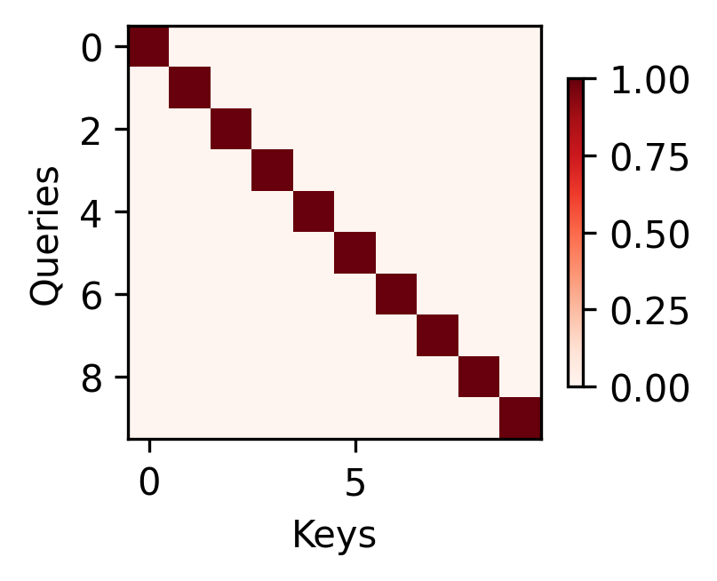
注意力的可视化
代码
import torch
from d2l import torch as d2l
from pathlib import Path

# 这个示例用于“看见”注意力权重矩阵:
# 1) 先构造一个可解释的注意力权重(这里用单位阵,表示每个 query 只关注同位置的 key)
# 2) 再把它绘制成热力图,颜色越深代表权重越大

def log_tensor_info(name, tensor):
    """打印张量的关键统计信息,便于理解可视化前的数据状态。"""
    print(f"[LOG] {name}:")
    print(f"      shape={tuple(tensor.shape)}, dtype={tensor.dtype}, device={tensor.device}")
    print(f"      min={tensor.min().item():.4f}, max={tensor.max().item():.4f}")
    print(f"      sum={tensor.sum().item():.4f}, non_zero={torch.count_nonzero(tensor).item()}")

#@save
def show_heatmaps(matrices, xlabel, ylabel, titles=None, figsize=(2.5, 2.5),
                  cmap='Reds', save_path='attention_heatmap.png'):
    """显示矩阵热图。

    参数 matrices 的形状通常为:
    (num_rows, num_cols, num_queries, num_keys)
    """
    log_tensor_info("输入到 show_heatmaps 的 matrices", matrices)

    d2l.use_svg_display()
    num_rows, num_cols = matrices.shape[0], matrices.shape[1]
    print(f"[LOG] 将创建子图网格: num_rows={num_rows}, num_cols={num_cols}")

    fig, axes = d2l.plt.subplots(num_rows, num_cols, figsize=figsize,
                                 sharex=True, sharey=True, squeeze=False)

    print("[LOG] 开始逐个子图绘制注意力矩阵...")
    for i, (row_axes, row_matrices) in enumerate(zip(axes, matrices)):
        for j, (ax, matrix) in enumerate(zip(row_axes, row_matrices)):
            # matrix 形状为 (num_queries, num_keys)
            print(
                f"[LOG] 绘制第 ({i}, {j}) 个注意力矩阵: "
                f"shape={tuple(matrix.shape)}, "
                f"row_sum(前3行)={matrix.sum(dim=-1)[:3].detach().numpy()}"
            )
            pcm = ax.imshow(matrix.detach().numpy(), cmap=cmap)
            if i == num_rows - 1:
                ax.set_xlabel(xlabel)
            if j == 0:
                ax.set_ylabel(ylabel)
            if titles:
                ax.set_title(titles[j])
    fig.colorbar(pcm, ax=axes, shrink=0.6)
    print("[LOG] 热力图绘制完成。颜色越深,表示该 query 对该 key 的注意力权重越高。")
    # 自动保存图片,便于离线查看和报告引用
    output_path = Path(save_path).resolve()
    fig.savefig(output_path, dpi=300, bbox_inches='tight')
    print(f"[LOG] 图片已自动保存到: {output_path}")

# 构造一个 10x10 的单位阵作为注意力矩阵:
# 对角线为 1,表示“自己最关注自己”;非对角线为 0,表示不关注其他位置。
attention_weights = torch.eye(10).reshape((1, 1, 10, 10))
log_tensor_info("attention_weights", attention_weights)

# 打印几行,直观看看每个 query 的分布
print("[LOG] attention_weights")
print(attention_weights)

# 触发可视化
show_heatmaps(attention_weights, xlabel='Keys', ylabel='Queries')
运行结果
[LOG] attention_weights
tensor([[[[1., 0., 0., 0., 0., 0., 0., 0., 0., 0.],
          [0., 1., 0., 0., 0., 0., 0., 0., 0., 0.],
          [0., 0., 1., 0., 0., 0., 0., 0., 0., 0.],
          [0., 0., 0., 1., 0., 0., 0., 0., 0., 0.],
          [0., 0., 0., 0., 1., 0., 0., 0., 0., 0.],
          [0., 0., 0., 0., 0., 1., 0., 0., 0., 0.],
          [0., 0., 0., 0., 0., 0., 1., 0., 0., 0.],
          [0., 0., 0., 0., 0., 0., 0., 1., 0., 0.],
          [0., 0., 0., 0., 0., 0., 0., 0., 1., 0.],
          [0., 0., 0., 0., 0., 0., 0., 0., 0., 1.]]]])
注意力汇聚:Nadaraya-Watson 核回归
为什么要有汇聚
汇聚 = 从“多个信息”得到“一个有用总结”
平均汇聚
代码
import torch
from torch import nn
from d2l import torch as d2l

n_train = 50  # 训练样本数
x_train, _ = torch.sort(torch.rand(n_train) * 5)   # 排序后的训练样本
print("模拟训练样本:")
print(x_train)

def f(x):
    return 2 * torch.sin(x) + x**0.8

y_train = f(x_train) + torch.normal(0.0, 0.5, (n_train,))  # 训练样本的输出
print("模拟训练样本输出:")
print(y_train)

x_test = torch.arange(0, 5, 0.1)  # 测试样本
print("模拟测试样本:")
print(x_test)

y_truth = f(x_test)  # 测试样本的真实输出
print("模拟测试样本真实输出:")
print(y_truth)

n_test = len(x_test)  # 测试样本数

def plot_kernel_reg(y_hat):
    d2l.plot(x_test, [y_truth, y_hat], 'x', 'y', legend=['Truth', 'Pred'],
             xlim=[0, 5], ylim=[-1, 5])
    d2l.plt.plot(x_train, y_train, 'o', alpha=0.5);
    d2l.plt.show()

y_hat = torch.repeat_interleave(y_train.mean(), n_test)
plot_kernel_reg(y_hat)
运行结果
模拟训练样本:
tensor([0.0186, 0.0420, 0.0634, 0.0708, 0.0996, 0.6909, 0.7262, 0.9220, 0.9588,
        0.9651, 1.0680, 1.1318, 1.2010, 1.2180, 1.2652, 1.2781, 1.5052, 1.5551,
        1.5922, 1.5924, 1.6596, 1.6799, 1.7515, 1.8087, 1.9410, 1.9650, 1.9928,
        2.1990, 2.2975, 2.7480, 2.8465, 2.9013, 3.0392, 3.1149, 3.4508, 3.4705,
        3.5038, 3.5831, 3.6419, 3.6621, 3.7065, 4.2261, 4.2504, 4.2622, 4.2973,
        4.3767, 4.3899, 4.5259, 4.6542, 4.9410])
模拟训练样本输出:
tensor([-0.2718, -0.4213,  0.8383,  0.2296, -0.1129,  1.9590,  2.7423,  1.6506,
         3.0730,  2.2361,  2.8086,  2.2452,  2.7972,  2.9973,  3.5080,  3.3284,
         3.2562,  3.2425,  4.0916,  3.8559,  3.0658,  4.0463,  3.6563,  3.7904,
         3.4871,  4.1421,  3.9534,  3.3734,  3.9171,  2.5372,  3.3241,  3.0082,
         2.4895,  2.4990,  2.3437,  2.1751,  2.1442,  1.2029,  1.5086,  1.9636,
         2.4231,  1.4694,  1.2094,  1.0402,  2.0655,  1.3921,  1.3843,  1.6869,
         1.7872,  1.3157])
模拟测试样本:
tensor([0.0000, 0.1000, 0.2000, 0.3000, 0.4000, 0.5000, 0.6000, 0.7000, 0.8000,
        0.9000, 1.0000, 1.1000, 1.2000, 1.3000, 1.4000, 1.5000, 1.6000, 1.7000,
        1.8000, 1.9000, 2.0000, 2.1000, 2.2000, 2.3000, 2.4000, 2.5000, 2.6000,
        2.7000, 2.8000, 2.9000, 3.0000, 3.1000, 3.2000, 3.3000, 3.4000, 3.5000,
        3.6000, 3.7000, 3.8000, 3.9000, 4.0000, 4.1000, 4.2000, 4.3000, 4.4000,
        4.5000, 4.6000, 4.7000, 4.8000, 4.9000])
模拟测试样本真实输出:
tensor([0.0000, 0.3582, 0.6733, 0.9727, 1.2593, 1.5332, 1.7938, 2.0402, 2.2712,
        2.4858, 2.6829, 2.8616, 3.0211, 3.1607, 3.2798, 3.3782, 3.4556, 3.5122,
        3.5481, 3.5637, 3.5597, 3.5368, 3.4960, 3.4385, 3.3654, 3.2783, 3.1787,
        3.0683, 2.9489, 2.8223, 2.6905, 2.5554, 2.4191, 2.2835, 2.1508, 2.0227,
        1.9013, 1.7885, 1.6858, 1.5951, 1.5178, 1.4554, 1.4089, 1.3797, 1.3684,
        1.3759, 1.4027, 1.4490, 1.5151, 1.6009])
训练数据
x_train:0 ~ 5 之间的随机点(已排序) y_train:真实函数 + 噪声
👉 特点:
有明显趋势(先升后降) 但噪声很大(±0.5)
测试数据(干净)
x_test:均匀分布(0 → 5) y_truth:真实函数(无噪声)
👉 这是你真正想拟合的目标
多项式回归和Attention
| 对比点 | 多项式回归 | Attention / 核回归 |
|---|---|---|
| 函数形式 | 固定(全局) | 动态(局部) |
| 参数 | 有限(w) | 数据驱动 |
| 表达能力 | 依赖阶数 | 自适应 |
| 对局部变化 | ❌ 差 | ✅ 强 |
多项式回归在做什么?
🔥 多项式
- 全局一个函数
- 所有 x 用同一套参数
- 必须选阶数(很敏感)
Attention是什么
🔥 Attention
- 每个 x 都是一个“局部模型”
- 权重随 x 变化
- 不需要预设函数形状
Attention 不是为了解决多项式训练难,而是提供了一种“完全不依赖函数假设”的建模方式。
平均汇聚的问题
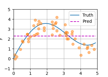
图里会看到:
- 蓝线(Truth)→ 真实函数(弯曲)
- 橙线(Pred)→ 一条水平直线
- 散点 → 带噪声训练数据
非参数注意力汇聚
代码
# X_repeat的形状:(n_test,n_train),
# 每一行都包含着相同的测试输入(例如:同样的查询)
X_repeat = x_test.repeat_interleave(n_train).reshape((-1, n_train))
# x_train包含着键。attention_weights的形状:(n_test,n_train),
# 每一行都包含着要在给定的每个查询的值(y_train)之间分配的注意力权重
attention_weights = nn.functional.softmax(-(X_repeat - x_train)**2 / 2, dim=1)
# y_hat的每个元素都是值的加权平均值,其中的权重是注意力权重
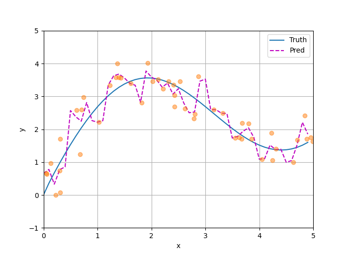
y_hat = torch.matmul(attention_weights, y_train)
plot_kernel_reg(y_hat)
如何理解
Nadaraya–Watson 核回归 = 用“相似度”作为权重,对训练样本做加权平均
Nadaraya–Watson 核回归(Kernel Regression) 是一种不依赖于预设函数形式(比如直线或二次曲线)的平滑技术。
构造 Query(X_repeat)
X_repeat = x_test.repeat_interleave(n_train).reshape((-1, n_train))
这一步展开的本质目的是为了实现“全连接”式的对比,将原本两个独立的向量,转化成一个能够覆盖所有组合的距离矩阵。
如果不进行这一步,你无法直接计算“每一个测试点”与“每一个训练点”之间的相互关系。
x_test:

tensor([0.0000, 0.1000, 0.2000, 0.3000, 0.4000, 0.5000, 0.6000, 0.7000, 0.8000,
        0.9000, 1.0000, 1.1000, 1.2000, 1.3000, 1.4000, 1.5000, 1.6000, 1.7000,
        1.8000, 1.9000, 2.0000, 2.1000, 2.2000, 2.3000, 2.4000, 2.5000, 2.6000,
        2.7000, 2.8000, 2.9000, 3.0000, 3.1000, 3.2000, 3.3000, 3.4000, 3.5000,
        3.6000, 3.7000, 3.8000, 3.9000, 4.0000, 4.1000, 4.2000, 4.3000, 4.4000,
        4.5000, 4.6000, 4.7000, 4.8000, 4.9000])

n_train = 50  # 训练样本数


X_repeat:
tensor([[0.0000, 0.0000, 0.0000,  ..., 0.0000, 0.0000, 0.0000],
        [0.1000, 0.1000, 0.1000,  ..., 0.1000, 0.1000, 0.1000],
        [0.2000, 0.2000, 0.2000,  ..., 0.2000, 0.2000, 0.2000],
        ...,
        [4.7000, 4.7000, 4.7000,  ..., 4.7000, 4.7000, 4.7000],
        [4.8000, 4.8000, 4.8000,  ..., 4.8000, 4.8000, 4.8000],
        [4.9000, 4.9000, 4.9000,  ..., 4.9000, 4.9000, 4.9000]])
Key(x_train)
模拟训练样本:
tensor([0.1418, 0.1642, 0.1750, 0.2202, 0.2541, 0.2821, 0.3730, 0.4815, 0.5860,
        0.6728, 0.9183, 1.0091, 1.1341, 1.3721, 1.4833, 1.4837, 1.5496, 1.5632,
        1.5910, 1.7081, 1.8227, 1.9113, 1.9441, 2.0197, 2.0671, 2.0725, 2.1231,
        2.1871, 2.2565, 2.2749, 2.5294, 2.5709, 2.5776, 2.9222, 3.0545, 3.1798,
        3.2841, 3.3407, 3.4414, 3.4944, 3.6850, 3.8908, 4.2214, 4.2682, 4.3725,
        4.5547, 4.5627, 4.6533, 4.8428, 4.9730])
[LOG] x_train: shape=(50,), dtype=torch.float32
      min=0.1418, max=4.9730, mean=2.2452
计算“相似度”(核心)
-(X_repeat - x_train)**2 / 2
-(X_repeat - x_train) ** 2 / 2 实际上是在计算 负的欧几里得距离平方。距离越小,计算结果越接近 0;距离越大,结果越小(负得越多)。
[LOG] key 的未归一化核分数):
      [-0.0100, -0.0274, -0.0744, ..., -10.2319, -10.4828, -12.4030]
      [-0.0009, -0.0090, -0.0408, ..., -9.7846, -10.0299, -11.9099]
      [-0.0017, -0.0006, -0.0172, ..., -9.3472, -9.5870, -11.4269]
      ...
      [-10.3894, -9.9729, -9.3068, ..., -0.0155, -0.0073, -0.0394]
      [-10.8502, -10.4245, -9.7432, ..., -0.0382, -0.0245, -0.0163]
      [-11.3210, -10.8861, -10.1897, ..., -0.0708, -0.0516, -0.0032]
softmax → 归一化权重
attention_weights = nn.functional.softmax(kernel_scores, dim=1)
归一后的矩阵:
[LOG] attention_weights:
      [0.0810, 0.0803, 0.0789, ..., 0.0000, 0.0000, 0.0000]
      [0.0751, 0.0749, 0.0743, ..., 0.0000, 0.0000, 0.0000]
      [0.0693, 0.0696, 0.0696, ..., 0.0000, 0.0000, 0.0000]
      ...
      [0.0000, 0.0000, 0.0000, ..., 0.0638, 0.0635, 0.0618]
      [0.0000, 0.0000, 0.0000, ..., 0.0668, 0.0678, 0.0669]
      [0.0000, 0.0000, 0.0000, ..., 0.0697, 0.0721, 0.0722]
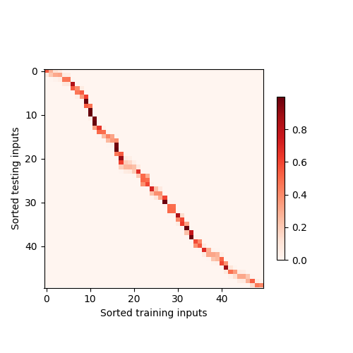
热力图

- 纵轴(Testing inputs): 你的每一个查询点(Query)。从上到下,对应测试样本从小到大(0 到 5)。
- 横轴(Training inputs): 你的每一个训练样本(Key)。从左到右,对应训练样本从小到大(0 到 5)。
- 颜色深浅: 代表 权重(Attention Weight) 的大小。颜色越深(或越亮,取决于色调),表示权重越高。
你会发现热力图中有一条非常明显的深色对角线,这揭示了核回归的本质:
- 局部性: 当测试点 $x$ 靠近某个训练点 $x_i$ 时,它们的距离最小,核分数最高,经过 Softmax 后的权重也就最大。
- 对角线意义: 因为你的测试集和训练集都排过序了。当纵坐标的测试点增加时,它离对应的横坐标训练点最近。所以深色块会随着测试点的增加而向右移动,形成对角线。
加权求和(最终预测)
y_hat = torch.matmul(attention_weights, y_train)
矩阵打印:
y_train:
tensor([1.1820, 0.9781, 0.4399, 1.3300, 1.1860, 1.2450, 2.3812, 2.4208, 2.8213, 2.5035,
        3.1059, 2.7856, 2.4552, 3.5986, 2.9405, 3.4057, 3.5368, 3.3820, 3.0238, 3.4779,
        4.1632, 3.2538, 3.7339, 3.9278, 4.1816, 2.7987, 2.5693, 3.7879, 3.8108, 2.9873,
        3.3099, 2.5070, 1.7757, 2.5167, 1.7410, 1.6363, 0.4733, 1.9042, 1.6949, 1.1083,
        2.4076, 1.1661, 1.4391, 2.0860, 0.5182, 1.7928, 1.0237, 1.5783, 0.8733, 1.1713])

[LOG] 前50个预测值 vs 真实值:
      x=0.00, pred=2.1060, truth=0.0000
      x=0.10, pred=2.1738, truth=0.3582
      x=0.20, pred=2.2415, truth=0.6733
      x=0.30, pred=2.3089, truth=0.9727
      x=0.40, pred=2.3754, truth=1.2593
      x=0.50, pred=2.4409, truth=1.5332
      x=0.60, pred=2.5048, truth=1.7938
      x=0.70, pred=2.5668, truth=2.0402
      x=0.80, pred=2.6266, truth=2.2712
      x=0.90, pred=2.6836, truth=2.4858
      x=1.00, pred=2.7376, truth=2.6829
      x=1.10, pred=2.7880, truth=2.8616
      x=1.20, pred=2.8344, truth=3.0211
      x=1.30, pred=2.8764, truth=3.1607
      x=1.40, pred=2.9137, truth=3.2798
      x=1.50, pred=2.9458, truth=3.3782
      x=1.60, pred=2.9722, truth=3.4556
      x=1.70, pred=2.9927, truth=3.5122
      x=1.80, pred=3.0070, truth=3.5481
      x=1.90, pred=3.0146, truth=3.5637
      x=2.00, pred=3.0154, truth=3.5597
      x=2.10, pred=3.0092, truth=3.5368
      x=2.20, pred=2.9959, truth=3.4960
      x=2.30, pred=2.9755, truth=3.4385
      x=2.40, pred=2.9481, truth=3.3654
      x=2.50, pred=2.9139, truth=3.2783
      x=2.60, pred=2.8732, truth=3.1787
      x=2.70, pred=2.8265, truth=3.0683
      x=2.80, pred=2.7745, truth=2.9489
      x=2.90, pred=2.7178, truth=2.8223
      x=3.00, pred=2.6572, truth=2.6905
      x=3.10, pred=2.5936, truth=2.5554
      x=3.20, pred=2.5279, truth=2.4191
      x=3.30, pred=2.4611, truth=2.2835
      x=3.40, pred=2.3941, truth=2.1508
      x=3.50, pred=2.3278, truth=2.0227
      x=3.60, pred=2.2629, truth=1.9013
      x=3.70, pred=2.2000, truth=1.7885
      x=3.80, pred=2.1398, truth=1.6858
      x=3.90, pred=2.0827, truth=1.5951
      x=4.00, pred=2.0289, truth=1.5178
      x=4.10, pred=1.9787, truth=1.4554
      x=4.20, pred=1.9321, truth=1.4089
      x=4.30, pred=1.8890, truth=1.3797
      x=4.40, pred=1.8495, truth=1.3684
      x=4.50, pred=1.8134, truth=1.3759
      x=4.60, pred=1.7805, truth=1.4027
      x=4.70, pred=1.7505, truth=1.4490
      x=4.80, pred=1.7232, truth=1.5151
      x=4.90, pred=1.6984, truth=1.6009

直观理解
🎯 对每个 x_test:“我应该相信哪些训练点?”
举个例子:x_test = 1.0
距离计算:
| x_train | 距离 | 权重 |
|---|---|---|
| 0.1 | 远 | 很小 |
| 0.9 | 近 | 很大 |
| 1.0 | 最近 | 最大 |
| 4.5 | 很远 | 接近0 |
👉 最终效果:只用“附近的点”来预测
注意力机制的雏形
你代码里用的 softmax,实际上是把核回归看作了一个“即时查表”的过程:
- Query(查询): 你的 x_test。
- Key(键): 你的 x_train。
- Value(值): 你的 y_train。
整个过程就是:计算查询与键的相似度(核分数),归一化成权重,然后对值进行加权求和。
带参数的注意力汇聚
# =========================
# 带参数的 Nadaraya-Watson 核回归
# =========================
# 上面“无参数”版本中,核函数宽度是固定的;
# 这里引入一个可学习参数 w,让模型自动学习“关注范围”:
# - |w| 大:距离被放大,softmax 更尖锐(更偏向局部邻近点)
# - |w| 小:距离被缩小,softmax 更平滑(会参考更远的点)
class NWKernelRegression(nn.Module):
def __init__(self, **kwargs):
super().__init__(**kwargs)
# 可学习的标量参数,用于缩放 queries 与 keys 的距离
# 训练会通过最小化预测误差自动更新它
self.w = nn.Parameter(torch.rand((1,), requires_grad=True))
def forward(self, queries, keys, values):
# 输入含义:
# queries: (查询个数,)
# keys: (查询个数, 每个查询可用的键数量)
# values: (查询个数, 每个查询可用的值数量) 其中数量与 keys 对齐
#
# 将 queries 按列复制,变成 (查询个数, 键数量),
# 以便逐元素计算每个 query 到所有 key 的距离
queries = queries.repeat_interleave(keys.shape[1]).reshape((-1, keys.shape[1]))
# 计算高斯核分数并做 softmax,得到注意力权重:
# score = -((q - k) * w)^2 / 2
# attention_weights 的每一行和为 1
self.attention_weights = nn.functional.softmax(
-((queries - keys) * self.w)**2 / 2, dim=1)
# 对 values 做加权求和,得到每个查询的预测值
# bmm 过程:
# - attention_weights.unsqueeze(1): (batch, 1, 键数量)
# - values.unsqueeze(-1): (batch, 键数量, 1)
# 输出: (batch, 1, 1) -> reshape(-1)
return torch.bmm(self.attention_weights.unsqueeze(1),
values.unsqueeze(-1)).reshape(-1)
# -------------------------
# 训练数据重排(留一法)
# -------------------------
# 对训练集中的第 i 个样本做预测时,不使用它自己作为 key/value,
# 否则模型会“偷看答案”(距离为 0 往往导致极高权重)。
# 因此我们构造一个 n_train x (n_train-1) 的键值表,每行都去掉对角元素。
# X_tile 的形状: (n_train, n_train),每一行都是完整的 x_train
X_tile = x_train.repeat((n_train, 1))
# Y_tile 的形状: (n_train, n_train),每一行都是完整的 y_train
Y_tile = y_train.repeat((n_train, 1))
# 使用布尔掩码去掉对角线元素,得到 leave-one-out 的 keys/values
# keys 的形状: (n_train, n_train - 1)
keys = X_tile[(1 - torch.eye(n_train)).type(torch.bool)].reshape((n_train, -1))
# values 的形状: (n_train, n_train - 1)
values = Y_tile[(1 - torch.eye(n_train)).type(torch.bool)].reshape((n_train, -1))
# 初始化模型、损失和优化器
net = NWKernelRegression()
print(f"[LOG] 初始权重参数 w = {net.w.item():.6f}")
# 不做 reduction,保留每个样本损失,便于后续灵活处理
loss = nn.MSELoss(reduction='none')
trainer = torch.optim.SGD(net.parameters(), lr=0.5)
animator = d2l.Animator(xlabel='epoch', ylabel='loss', xlim=[1, 5])
# 训练阶段:让模型学到合适的 w,使训练集预测误差尽可能小
for epoch in range(5):
trainer.zero_grad()
# 对每个训练样本,用“其余 n_train-1 个样本”作为键值库做预测
l = loss(net(x_train, keys, values), y_train)
# 将逐样本损失求和,得到标量目标用于反向传播
l.sum().backward()
trainer.step()
print(f'epoch {epoch + 1}, loss {float(l.sum()):.6f}, w {net.w.item():.6f}')
animator.add(epoch + 1, float(l.sum()))
print(f"[LOG] 训练结束后的权重参数 w = {net.w.item():.6f}")
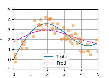
# -------------------------
# 测试阶段预测
# -------------------------
# 测试时没有“标签泄漏”问题,因此每个测试 query 都可使用完整训练集作为键值库。
# keys 的形状: (n_test, n_train),每一行都是完整训练输入 x_train
keys = x_train.repeat((n_test, 1))
# values 的形状: (n_test, n_train),每一行都是完整训练输出 y_train
values = y_train.repeat((n_test, 1))
# 得到测试集预测;unsqueeze(1) 仅用于和绘图函数输入对齐
y_hat = net(x_test, keys, values).unsqueeze(1).detach()
plot_kernel_reg(y_hat)
d2l.plt.show()
运行结果
[LOG] 初始权重参数 w = 0.759302
epoch 1, loss 38.602791, w 19.008167
epoch 2, loss 15.362171, w 18.982002
epoch 3, loss 15.360804, w 18.955769
epoch 4, loss 15.359426, w 18.929468
epoch 5, loss 15.358039, w 18.903099
[LOG] 训练结束后的权重参数 w = 18.903099
w 到底在干什么?
带参数的核分数(Kernel Score)
\[\text{score}_i = -\frac{((x - x_i) \cdot w)^2}{2}\]在公式 score = -((queries - keys) * self.w)**2 / 2 中,$w$ 扮演的是缩放因子(Scaling factor)的角色:
-
如果 $ w $ 很大: 哪怕 $x$ 和 $x_i$ 只有一点点距离,乘以 $w$ 后距离也会被放大。这意味着核函数变得非常“尖锐”,模型只关注极近的邻居。 -
如果 $ w $ 很小: 距离被缩小,核函数变得非常“平滑”,模型会变得“大方”,参考较远的邻居。
注意力权重(Attention Weights)
通过 softmax 函数,将上面的分数转化为归一化的权重(概率分布),确保所有权重之和为 1:
\[w(x, x_i) = \frac{\exp(\text{score}_i)}{\sum_{j=1}^{n} \exp(\text{score}_j)}\]- 这个公式决定了在预测 $x$ 时,每一个训练观测值 $y_i$ 应该占多大的比例。
- 当 $w$ 很大时,这个分布会变得非常“尖锐”(集中在最近的点上);当 $w$ 很小时,分布会变得“平坦”。
最终预测值(Final Prediction)
预测值 $y$ 是所有训练标签 $y_i$ 的加权平均,这在代码中对应 torch.bmm 或 torch.matmul:
\[\hat{y} = \sum_{i=1}^{n} w(x, x_i) \cdot y_i\]热力图
注意力评分函数
高斯核指数部分可以视为注意力评分函数(attention scoring function), 简称评分函数(scoring function), 然后把这个函数的输出结果输入到softmax函数中进行运算。
通过上述步骤,将得到与键对应的值的概率分布(即注意力权重)。 最后,注意力汇聚的输出就是基于这些注意力权重的值的加权和。

加性注意力评分函数
核心公式
加性注意力评分函数通常定义为:
\[a(\mathbf{q}, \mathbf{k}) = \mathbf{v}^\top \text{tanh}(\mathbf{W}_q \mathbf{q} + \mathbf{W}_k \mathbf{k})\]这里不再只有一个参数 $w$,而是引入了三组矩阵/向量:
- $\mathbf{W}_q$ 和 $\mathbf{W}_k$:将查询(Query)和键(Key)映射到相同的隐藏维度。
- $\text{tanh}$:非线性激活函数,增加模型的表达能力。
- $\mathbf{v}$:一个权重向量,将隐藏表示压缩成一个标量分值。
代码
import torch
from torch import nn
from d2l import torch as d2l

def log_tensor(name, tensor):
    """打印张量形状与全部元素,便于完整查看数据流。"""
    print(f"[LOG] {name}: shape={tuple(tensor.shape)}, dtype={tensor.dtype}")
    print(tensor)

#@save
def masked_softmax(X, valid_lens):
    """通过在最后一个轴上掩蔽元素来执行softmax操作"""
    # X:3D张量,valid_lens:1D或2D张量
    print("\n[LOG] 进入 masked_softmax")
    log_tensor("masked_softmax 输入 X", X)
    if valid_lens is not None:
        log_tensor("masked_softmax 输入 valid_lens", valid_lens)

    if valid_lens is None:
        print("[LOG] valid_lens=None,不做掩码,直接 softmax。")
        return nn.functional.softmax(X, dim=-1)
    else:
        shape = X.shape
        print(f"[LOG] X 原始形状={shape}")
        if valid_lens.dim() == 1:
            print("[LOG] valid_lens 是 1D,按查询数复制,使其和 X 的前两维对齐。")
            valid_lens = torch.repeat_interleave(valid_lens, shape[1])
        else:
            print("[LOG] valid_lens 是 2D,先 reshape 成 1D。")
            valid_lens = valid_lens.reshape(-1)
        log_tensor("展开后的 valid_lens", valid_lens)

        # 最后一轴上被掩蔽的元素使用一个非常大的负值替换,从而其softmax输出为0
        X = d2l.sequence_mask(X.reshape(-1, shape[-1]), valid_lens,
                              value=-1e6)
        log_tensor("掩码后的 X(被遮挡位置约为 -1e6)", X)
        out = nn.functional.softmax(X.reshape(shape), dim=-1)
        log_tensor("masked_softmax 输出", out)
        return out

#@save
class AdditiveAttention(nn.Module):
    """加性注意力"""
    def __init__(self, key_size, query_size, num_hiddens, dropout, **kwargs):
        super(AdditiveAttention, self).__init__(**kwargs)
        # 将 key/query 映射到同一隐藏空间,便于可加地比较“匹配程度”
        self.W_k = nn.Linear(key_size, num_hiddens, bias=False)
        self.W_q = nn.Linear(query_size, num_hiddens, bias=False)
        # 将 tanh 后的特征压缩为单个分数(每个 query-key 对应一个 score)
        self.w_v = nn.Linear(num_hiddens, 1, bias=False)
        self.dropout = nn.Dropout(dropout)

    def forward(self, queries, keys, values, valid_lens):
        print("\n[LOG] ====== AdditiveAttention.forward 开始 ======")
        log_tensor("输入 queries", queries)
        log_tensor("输入 keys", keys)
        log_tensor("输入 values", values)
        log_tensor("输入 valid_lens", valid_lens)

        queries, keys = self.W_q(queries), self.W_k(keys)
        log_tensor("线性变换后 queries=W_q(queries)", queries)
        log_tensor("线性变换后 keys=W_k(keys)", keys)
        # 在维度扩展后,
        # queries的形状:(batch_size,查询的个数,1,num_hidden)
        # key的形状:(batch_size,1,“键-值”对的个数,num_hiddens)
        # 使用广播方式进行求和
        features = queries.unsqueeze(2) + keys.unsqueeze(1)
        log_tensor("广播求和后 features", features)
        features = torch.tanh(features)
        log_tensor("tanh 激活后 features", features)
        # self.w_v仅有一个输出,因此从形状中移除最后那个维度。
        # scores的形状:(batch_size,查询的个数,“键-值”对的个数)
        scores = self.w_v(features).squeeze(-1)
        log_tensor("注意力打分 scores", scores)
        self.attention_weights = masked_softmax(scores, valid_lens)
        log_tensor("注意力权重 attention_weights", self.attention_weights)
        print(f"[LOG] 权重按 key 维求和(应接近 1):\n{self.attention_weights.sum(dim=-1)}")
        # values的形状:(batch_size,“键-值”对的个数,值的维度)
        out = torch.bmm(self.dropout(self.attention_weights), values)
        log_tensor("加权求和输出 out", out)
        print("[LOG] ====== AdditiveAttention.forward 结束 ======\n")
        return out

queries, keys = torch.normal(0, 1, (2, 1, 20)), torch.ones((2, 10, 2))
# values的小批量,两个值矩阵是相同的
values = torch.arange(40, dtype=torch.float32).reshape(1, 10, 4).repeat(
    2, 1, 1)
valid_lens = torch.tensor([2, 6])

attention = AdditiveAttention(key_size=2, query_size=20, num_hiddens=8,
                              dropout=0.1)
attention.eval()
out = attention(queries, keys, values, valid_lens)
print("[LOG] 最终输出 out:")
print(out)
print("[LOG] 最终注意力权重 attention.attention_weights:")
print(attention.attention_weights)
模型权重参数
[LOG] W_k 权重矩阵: shape=(8, 2), dtype=torch.float32
Parameter containing:
tensor([[ 0.5079,  0.2072],
        [-0.0737,  0.4615],
        [-0.0524,  0.2056],
        [ 0.5446,  0.0680],
        [ 0.4575, -0.3793],
        [ 0.2400,  0.0051],
        [-0.1360, -0.3073],
        [ 0.0923, -0.3941]], requires_grad=True)
[LOG] W_q 权重矩阵: shape=(8, 20), dtype=torch.float32
Parameter containing:
tensor([[-0.1981, -0.0482,  0.0008,  0.1674, -0.1539,  0.1084,  0.0889, -0.2041,
          0.0319,  0.1609, -0.1887, -0.0132,  0.0623,  0.1151,  0.1884, -0.0775,
         -0.0468,  0.1427,  0.0332,  0.1167],
        [ 0.1562,  0.0731, -0.1485, -0.1873, -0.0920,  0.1551,  0.2091, -0.0053,
          0.0243,  0.0453,  0.0456,  0.1236, -0.1930,  0.0318, -0.1040,  0.0409,
          0.2102,  0.1306, -0.1730,  0.0082],
        [-0.1465,  0.0117, -0.2219,  0.0349, -0.0039,  0.0120,  0.1167, -0.2163,
         -0.1185, -0.0799, -0.0210, -0.0671,  0.1861,  0.1190,  0.0241, -0.1276,
         -0.1570, -0.1735,  0.1607, -0.0730],
        [-0.1013, -0.0026, -0.1240, -0.0055, -0.1456,  0.0137,  0.1853, -0.1863,
          0.0553,  0.0287,  0.0476, -0.0671,  0.0292, -0.0608, -0.0844, -0.0455,
          0.0840,  0.0242,  0.1991, -0.0279],
        [-0.1793, -0.1896,  0.1575, -0.1299,  0.2113,  0.1866, -0.0035,  0.2033,
          0.0667,  0.1738, -0.1495, -0.1226,  0.1690, -0.1725,  0.1673, -0.0523,
          0.1190,  0.0652,  0.0973, -0.1520],
        [ 0.1134, -0.0499,  0.1912, -0.1787, -0.1198,  0.0860, -0.0496,  0.1757,
         -0.2236, -0.0785,  0.1071, -0.0147, -0.0271,  0.1872,  0.1206,  0.1478,
          0.0734,  0.0887,  0.1312, -0.0356],
        [-0.0457,  0.1873,  0.0289,  0.1103,  0.0287, -0.2004,  0.0466, -0.2040,
         -0.1749,  0.0392,  0.0266, -0.2130, -0.1863,  0.1892, -0.1188,  0.0809,
         -0.0900,  0.1937,  0.1648,  0.1382],
        [-0.1682,  0.0352, -0.1980, -0.0869,  0.1459, -0.1284, -0.1702, -0.1344,
          0.0012,  0.1193, -0.1805,  0.1122,  0.1198,  0.0857, -0.0409,  0.1526,
         -0.1087, -0.1504,  0.0270, -0.1385]], requires_grad=True)
[LOG] w_v 权重矩阵: shape=(1, 8), dtype=torch.float32
Parameter containing:
tensor([[-0.2879,  0.2746,  0.0657,  0.1356,  0.3156,  0.1146, -0.2173, -0.0852]],
       requires_grad=True)
输入结构
queries: (2, 1, 20)
keys:    (2, 10, 2)
values:  (2, 10, 4)
valid_lens: [2, 6]

每个样本:
拿一个问题(query)
去10个候选(keys)里找最相关的
然后取对应的信息(values)

[LOG] 输入 queries: shape=(2, 1, 20), dtype=torch.float32
tensor([[[ 0.2064, -0.5376,  0.8412, -0.2751,  1.0507,  1.6315, -0.3984,
          -1.1002,  0.5032, -1.5185,  2.2012, -0.3228,  1.0441,  1.2034,
          -0.9684,  0.4013, -0.6058,  0.9404,  0.4188, -0.5444]],

        [[ 0.6491, -1.1137, -0.0694,  1.0564,  1.6361, -0.7537,  0.5378,
           0.8582, -1.5430,  0.2189,  0.0728, -0.3820,  1.4850,  0.7147,
          -1.2918,  0.9103, -0.3724,  0.3866, -0.6202,  0.3237]]])
[LOG] 输入 keys: shape=(2, 10, 2), dtype=torch.float32
tensor([[[1., 1.],
         [1., 1.],
         [1., 1.],
         [1., 1.],
         [1., 1.],
         [1., 1.],
         [1., 1.],
         [1., 1.],
         [1., 1.],
         [1., 1.]],

        [[1., 1.],
         [1., 1.],
         [1., 1.],
         [1., 1.],
         [1., 1.],
         [1., 1.],
         [1., 1.],
         [1., 1.],
         [1., 1.],
         [1., 1.]]])
[LOG] 输入 values: shape=(2, 10, 4), dtype=torch.float32
tensor([[[ 0.,  1.,  2.,  3.],
         [ 4.,  5.,  6.,  7.],
         [ 8.,  9., 10., 11.],
         [12., 13., 14., 15.],
         [16., 17., 18., 19.],
         [20., 21., 22., 23.],
         [24., 25., 26., 27.],
         [28., 29., 30., 31.],
         [32., 33., 34., 35.],
         [36., 37., 38., 39.]],

        [[ 0.,  1.,  2.,  3.],
         [ 4.,  5.,  6.,  7.],
         [ 8.,  9., 10., 11.],
         [12., 13., 14., 15.],
         [16., 17., 18., 19.],
         [20., 21., 22., 23.],
         [24., 25., 26., 27.],
         [28., 29., 30., 31.],
         [32., 33., 34., 35.],
         [36., 37., 38., 39.]]])
| 名字 | 含义 |
|---|---|
| batch=2 | 两个样本 |
| query数=1 | 每个样本只查一次 |
| key数=10 | 有10个候选 |
| value维度=4 | 每个key对应一个4维输出 |
线性变换(统一空间)
      queries, keys = self.W_q(queries), self.W_k(keys)

[LOG] 线性变换后 queries=W_q(queries): shape=(2, 1, 8), dtype=torch.float32
tensor([[[-0.0809, -0.7336,  0.9886, -0.0700,  0.6035,  0.0832, -0.9505, 0.0988]],
        [[-0.2756, -0.8232, -0.1916, -0.6070,  0.3838,  0.0319, -0.3750, 0.4496]]], grad_fn=<UnsafeViewBackward0>)
[LOG] 线性变换后 keys=W_k(keys): shape=(2, 10, 8), dtype=torch.float32
tensor([[[ 0.7151,  0.3878,  0.1532,  0.6126,  0.0783,  0.2451, -0.4433, -0.3018],
         [ 0.7151,  0.3878,  0.1532,  0.6126,  0.0783,  0.2451, -0.4433, -0.3018],
         [ 0.7151,  0.3878,  0.1532,  0.6126,  0.0783,  0.2451, -0.4433, -0.3018],
         [ 0.7151,  0.3878,  0.1532,  0.6126,  0.0783,  0.2451, -0.4433, -0.3018],
         [ 0.7151,  0.3878,  0.1532,  0.6126,  0.0783,  0.2451, -0.4433, -0.3018],
         [ 0.7151,  0.3878,  0.1532,  0.6126,  0.0783,  0.2451, -0.4433, -0.3018],
         [ 0.7151,  0.3878,  0.1532,  0.6126,  0.0783,  0.2451, -0.4433, -0.3018],
         [ 0.7151,  0.3878,  0.1532,  0.6126,  0.0783,  0.2451, -0.4433, -0.3018],
         [ 0.7151,  0.3878,  0.1532,  0.6126,  0.0783,  0.2451, -0.4433, -0.3018],
         [ 0.7151,  0.3878,  0.1532,  0.6126,  0.0783,  0.2451, -0.4433, -0.3018],

        [[ 0.7151,  0.3878,  0.1532,  0.6126,  0.0783,  0.2451, -0.4433, -0.3018],
         [ 0.7151,  0.3878,  0.1532,  0.6126,  0.0783,  0.2451, -0.4433, -0.3018],
         [ 0.7151,  0.3878,  0.1532,  0.6126,  0.0783,  0.2451, -0.4433, -0.3018],
         [ 0.7151,  0.3878,  0.1532,  0.6126,  0.0783,  0.2451, -0.4433, -0.3018],
         [ 0.7151,  0.3878,  0.1532,  0.6126,  0.0783,  0.2451, -0.4433, -0.3018],
         [ 0.7151,  0.3878,  0.1532,  0.6126,  0.0783,  0.2451, -0.4433, -0.3018],
         [ 0.7151,  0.3878,  0.1532,  0.6126,  0.0783,  0.2451, -0.4433, -0.3018],
         [ 0.7151,  0.3878,  0.1532,  0.6126,  0.0783,  0.2451, -0.4433, -0.3018],
         [ 0.7151,  0.3878,  0.1532,  0.6126,  0.0783,  0.2451, -0.4433, -0.3018],
         [ 0.7151,  0.3878,  0.1532,  0.6126,  0.0783,  0.2451, -0.4433, -0.3018]]], grad_fn=<UnsafeViewBackward0>)
广播 + 相加
[LOG] 广播求和后 features: shape=(2, 1, 10, 8), dtype=torch.float32
tensor([[[[ 0.6343, -0.3458,  1.1419,  0.5425,  0.6818,  0.3282, -1.3938, -0.2030],
          [ 0.6343, -0.3458,  1.1419,  0.5425,  0.6818,  0.3282, -1.3938, -0.2030],
          [ 0.6343, -0.3458,  1.1419,  0.5425,  0.6818,  0.3282, -1.3938, -0.2030],
          [ 0.6343, -0.3458,  1.1419,  0.5425,  0.6818,  0.3282, -1.3938, -0.2030],
          [ 0.6343, -0.3458,  1.1419,  0.5425,  0.6818,  0.3282, -1.3938, -0.2030],
          [ 0.6343, -0.3458,  1.1419,  0.5425,  0.6818,  0.3282, -1.3938, -0.2030],
          [ 0.6343, -0.3458,  1.1419,  0.5425,  0.6818,  0.3282, -1.3938, -0.2030],
          [ 0.6343, -0.3458,  1.1419,  0.5425,  0.6818,  0.3282, -1.3938, -0.2030],
          [ 0.6343, -0.3458,  1.1419,  0.5425,  0.6818,  0.3282, -1.3938, -0.2030],
          [ 0.6343, -0.3458,  1.1419,  0.5425,  0.6818,  0.3282, -1.3938, -0.2030]]],


        [[[ 0.4395, -0.4354, -0.0384,  0.0056,  0.4621,  0.2770, -0.8183, 0.1478],
          [ 0.4395, -0.4354, -0.0384,  0.0056,  0.4621,  0.2770, -0.8183, 0.1478],
          [ 0.4395, -0.4354, -0.0384,  0.0056,  0.4621,  0.2770, -0.8183, 0.1478],
          [ 0.4395, -0.4354, -0.0384,  0.0056,  0.4621,  0.2770, -0.8183, 0.1478],
          [ 0.4395, -0.4354, -0.0384,  0.0056,  0.4621,  0.2770, -0.8183, 0.1478],
          [ 0.4395, -0.4354, -0.0384,  0.0056,  0.4621,  0.2770, -0.8183, 0.1478],
          [ 0.4395, -0.4354, -0.0384,  0.0056,  0.4621,  0.2770, -0.8183, 0.1478],
          [ 0.4395, -0.4354, -0.0384,  0.0056,  0.4621,  0.2770, -0.8183, 0.1478],
          [ 0.4395, -0.4354, -0.0384,  0.0056,  0.4621,  0.2770, -0.8183, 0.1478],
          [ 0.4395, -0.4354, -0.0384,  0.0056,  0.4621,  0.2770, -0.8183, 0.1478]]]], grad_fn=<AddBackward0>)
tanh + 线性 → 得到分数
[LOG] tanh 激活后 features: shape=(2, 1, 10, 8), dtype=torch.float32
tensor([[[[ 0.5610, -0.3326,  0.8150,  0.4949,  0.5927,  0.3169, -0.8840, -0.2003],
          [ 0.5610, -0.3326,  0.8150,  0.4949,  0.5927,  0.3169, -0.8840, -0.2003],
          [ 0.5610, -0.3326,  0.8150,  0.4949,  0.5927,  0.3169, -0.8840, -0.2003],
          [ 0.5610, -0.3326,  0.8150,  0.4949,  0.5927,  0.3169, -0.8840, -0.2003],
          .......
          [ 0.5610, -0.3326,  0.8150,  0.4949,  0.5927,  0.3169, -0.8840, -0.2003]]],


        [[[ 0.4132, -0.4098, -0.0384,  0.0056,  0.4318,  0.2701, -0.6741, 0.1467],
          [ 0.4132, -0.4098, -0.0384,  0.0056,  0.4318,  0.2701, -0.6741, 0.1467],
          [ 0.4132, -0.4098, -0.0384,  0.0056,  0.4318,  0.2701, -0.6741, 0.1467],
          .......
          [ 0.4132, -0.4098, -0.0384,  0.0056,  0.4318,  0.2701, -0.6741, 0.1467]]]], grad_fn=<TanhBackward0>)

[LOG] 注意力打分 scores: shape=(2, 1, 10), dtype=torch.float32
tensor([[[0.3003, 0.3003, 0.3003, 0.3003, 0.3003, 0.3003, 0.3003, 0.3003, 0.3003, 0.3003]],

        [[0.0679, 0.0679, 0.0679, 0.0679, 0.0679, 0.0679, 0.0679, 0.0679, 0.0679, 0.0679]]], grad_fn=<SqueezeBackward1>)
masked_softmax
[LOG] masked_softmax 输出: shape=(2, 1, 10), dtype=torch.float32
tensor([[[0.5000, 0.5000, 0.0000, 0.0000, 0.0000, 0.0000, 0.0000, 0.0000,
          0.0000, 0.0000]],

        [[0.1667, 0.1667, 0.1667, 0.1667, 0.1667, 0.1667, 0.0000, 0.0000,
          0.0000, 0.0000]]], grad_fn=<SoftmaxBackward0>)
最终输出
[LOG] 加权求和输出 out: shape=(2, 1, 4), dtype=torch.float32
tensor([[[ 2.0000,  3.0000,  4.0000,  5.0000]],
        [[10.0000, 11.0000, 12.0000, 13.0000]]], grad_fn=<BmmBackward0>)
总结
AdditiveAttention 是一个“带参数的神经网络层(Layer)”,用于计算注意力权重并进行加权汇聚。
理解 Additive Attention(加性注意力),你可以把它想象成一场“相亲大会上的匹配度打分”。
在这个场景里,有三个角色:
- Query(查询): 正在找对象的你。
- Key(键): 对方贴在背后的“个人简历”。
- Value(值): 对方真正的“内在性格/才华”(也就是你最终想获取的信息)。
第一步:统一语言(线性变换 $W_q$ 和 $W_k$)
假设你(Query)只会说中文,而对方的简历(Key)是用英文写的。你们直接沟通肯定会鸡同鸭讲。
- $W_q$:相当于给你请了一个翻译,把你感兴趣的特质转换成一种“通用特征空间”。
- $W_k$:给对方也请了一个翻译,把简历也转换成同样的“通用特征空间”。
现在,你们终于可以用同一种语言交流了。
第二步:加性结合(加法运算)
这是“加性”二字的由来。
模型把你的需求和对方的简历直接“拼”在了一起。想象你列了一个清单,对方也列了一个清单,模型把这两份清单叠在一起看:
你的需求 + 对方的条件 = 你们的共同话题
这就是代码里的 queries.unsqueeze(2) + keys.unsqueeze(1)。它把每一个 Query 和每一个 Key 都强行配对,看看它们加在一起产生的“化学反应”如何。
第三步:深度观察(tanh 与 $w_v$)
直接相加可能还是比较生硬。
- tanh 激活函数:相当于评审员。它会观察你们相加后的结果,把那些特别匹配的特征放大,把不匹配的特征缩小。
- w_v 线性层:这是一个打分员。他看着你们经过变换后的共同特质,最后给出一个具体的分数值(Score)。分数越高,说明你越看重这个对象。
第四步:屏蔽干扰(Masked Softmax)
在相亲会上,有些人可能是来凑数的(Padding/填充字符)。
- Masking:系统会自动给这些凑数的人打一个极低的分(比如负一百万分)。
- Softmax:把所有人的分数转化成百分比。因为凑数的人分极低,他们的百分比就是 0%。剩下的所有“有效对象”的百分比加起来等于 100%。
第五步:带走信息(加权求和)
最后,你并不是只带走一个人的信息。你是根据刚刚算的百分比(权重),去提取所有人的“才华”(Value)。
- 如果你对 1 号对象的注意力是 80%,对 2 号是 20%。
- 那你最终拿走的“印象”就是:80% 的 1 号才华 + 20% 的 2 号才华。
缩放点积注意力
缩放点积注意力(scaled dot-product attention)评分函数为:
\[Attention(Q, K, V) = \text{softmax}\left(\frac{Q \cdot K^T}{\sqrt{d_k}}\right)V\]它通过计算 Q 和 K 的夹角余弦(点积)来衡量相似度,并除以一个缩放因子。
这个公式里全是数学行为。它不学习任何东西,它只负责分配权重。如果 $Q, K, V$ 是固定不变的,那么无论运行多少遍,结果都是死板的。
Q --------\
           \         (相似度)      (归一化)      (加权)
            --> QK^T ---> /√d ---> softmax ---> × V ---> 输出
K --------/

V ------------------------------------------/
Attention 核心计算 = 纯算子,没有参数
第一步:$Q K^T$ —— “算匹配度”
在 Transformer 中,我们通常不是处理一个词,而是一次处理一整句话(一个矩阵)。
- $Q$ 矩阵:每一行代表一个“需求”。
- $K^T$ 矩阵:每一列代表一个“被查询的标签”。
当 $Q$ 乘以 $K^T$ 时:
- 矩阵乘法的本质是 $Q$ 的每一行去和 $K^T$ 的每一列做点积。
- 这就像是让每一个需求都去和每一个标签挨个碰一遍,算出一张巨大的“评分表”。
第二步:$/\sqrt{d_k}$ —— “降温降噪”
为什么要选“维度的平方根”,而不是除以 10 或者除以 $d_k$ 本身?这背后有一个精妙的统计学原因:
假设 $Q$ 和 $K$ 中的每一个数字都是符合标准正态分布的(均值为 0,方差为 1):
- 当你把两个长度为 $d_k$ 的向量做点积时,结果的均值依然是 0,但方差会变成 $d_k$。
- 这意味着,维度越高,点积算出来的分值波动就越大。有些分值会变得极大,有些极小。
- 方差太大对 Softmax 是致命的:如果输入 Softmax 的数值很大,梯度的模长会变得极小,导致模型在训练时“学不动了”(梯度消失)。
除以 $\sqrt{d_k}$ 的目的,就是把方差重新拉回到 1。 这样无论你把模型做得多宽(维度多大),进入 Softmax 的数据始终保持在一个“温和”的范围内。
第三步:$\text{softmax}(\dots) V$ —— “按比例分配工作”
\(\text{输出} = \text{权重}_1 \cdot V_1 + \text{权重}_2 \cdot V_2 + \dots + \text{权重}_n \cdot V_n\)这一步被称为“加权求和”。
对比
| 维度 | 加性注意力(Additive / Bahdanau) | 缩放点积注意力(Scaled Dot-Product) |
|---|---|---|
| 提出者 | Dzmitry Bahdanau | Attention Is All You Need |
| 核心思想 | 用小型神经网络算相关性 | 用向量点积算相似度 |
| 计算方式 | (w^T \tanh(W_q Q + W_k K)) | (QK^T / \sqrt{d_k}) |
| 是否有额外参数 | ✅ 有(MLP参数) | ❌ 无(本体无参数) |
| 表达能力 | ⭐ 更强(非线性) | ⭐⭐ 足够强(线性) |
| 计算速度 | ❌ 慢 | ✅ 很快 |
| 并行能力 | ❌ 差(逐对计算) | ✅ 强(矩阵乘法) |
| GPU/TPU友好 | ❌ 一般 | ✅ 极好 |
| 高维稳定性 | ✅ 稳定 | ⚠️ 需缩放(√d) |
| 是否需要缩放 | ❌ 不需要 | ✅ 必须 |
| 适合场景 | 小模型 / 早期Seq2Seq | 大模型 / Transformer |
| 工业使用 | ❌ 较少 | ✅ 主流(GPT/BERT/ViT) |
| 本质理解 | 学习一个“相似度函数” | 直接用“相似度计算” |
| 类比 | 面试官综合评估 | 搜索引擎关键词匹配 |